
13.4: Tangent Planes, Linear Approximations, and the Total Differential


( \newcommand{\kernel}{\mathrm{null}\,}\)
- Determine the equation of a plane tangent to a given surface at a point.
- Use the tangent plane to approximate a function of two variables at a point.
- Explain when a function of two variables is differentiable.
- Use the total differential to approximate the change in a function of two variables.
In this section, we consider the problem of finding the tangent plane to a surface, which is analogous to finding the equation of a tangent line to a curve when the curve is defined by the graph of a function of one variable, y=f(x). The slope of the tangent line at the point x=a is given by m=f′(a); what is the slope of a tangent plane? We learned about the equation of a plane in Equations of Lines and Planes in Space; in this section, we see how it can be applied to the problem at hand.
Tangent Planes
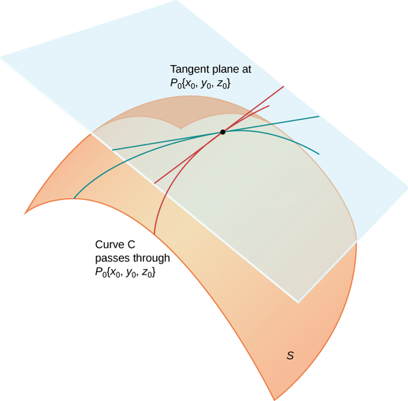
Intuitively, it seems clear that, in a plane, only one line can be tangent to a curve at a point. However, in three-dimensional space, many lines can be tangent to a given point. If these lines lie in the same plane, they determine the tangent plane at that point. A more intuitive way to think of a tangent plane is to assume the surface is smooth at that point (no corners). Then, a tangent line to the surface at that point in any direction does not have any abrupt changes in slope because the direction changes smoothly. Therefore, in a small-enough neighborhood around the point, a tangent plane touches the surface at that point only.
Let P0=(x0,y0,z0) be a point on a surface S, and let C be any curve passing through P0 and lying entirely in S. If the tangent lines to all such curves C at P0 lie in the same plane, then this plane is called the tangent plane to S at P0 (Figure 13.4.1).
For a tangent plane to a surface to exist at a point on that surface, it is sufficient for the function that defines the surface to be differentiable at that point. We define the term tangent plane here and then explore the idea intuitively.
Let S be a surface defined by a differentiable function z=f(x,y), and let P0=(x0,y0) be a point in the domain of f. Then, the equation of the tangent plane to S at P0 is given by
z=f(x0,y0)+fx(x0,y0)(x−x0)+fy(x0,y0)(y−y0).
To see why this formula is correct, let’s first find two tangent lines to the surface S. The equation of the tangent line to the curve that is represented by the intersection of S with the vertical trace given by x=x0 is z=f(x0,y0)+fy(x0,y0)(y−y0). Similarly, the equation of the tangent line to the curve that is represented by the intersection of S with the vertical trace given by y=y0 is z=f(x0,y0)+fx(x0,y0)(x−x0). A parallel vector to the first tangent line is ⇀a=ˆj+fy(x0,y0)ˆk; a parallel vector to the second tangent line is ⇀b=ˆi+fx(x0,y0)ˆk. We can take the cross product of these two vectors:
⇀a×⇀b=(ˆj+fy(x0,y0)ˆk)×(ˆi+fx(x0,y0)ˆk)=|ˆiˆjˆk01fy(x0,y0)10fx(x0,y0)|=fx(x0,y0)ˆi+fy(x0,y0)ˆj−ˆk.
This vector is perpendicular to both lines and is therefore perpendicular to the tangent plane. We can use this vector as a normal vector to the tangent plane, along with the point P0=(x0,y0,f(x0,y0)) in the equation for a plane:
⇀n·((x−x0)ˆi+(y−y0)ˆj+(z−f(x0,y0))ˆk)=0(fx(x0,y0)ˆi+fy(x0,y0)ˆj−ˆk)·((x−x0)ˆi+(y−y0)ˆj+(z−f(x0,y0))ˆk)=0fx(x0,y0)(x−x0)+fy(x0,y0)(y−y0)−(z−f(x0,y0))=0.
Solving this equation for z gives Equation ???.
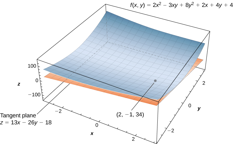
Find the equation of the tangent plane to the surface defined by the function f(x,y)=2x2−3xy+8y2+2x−4y+4 at point (2,−1).
Solution
First, we must calculate fx(x,y) and fy(x,y), then use Equation with x0=2 and y0=−1:
fx(x,y)=4x−3y+2fy(x,y)=−3x+16y−4f(2,−1)=2(2)2−3(2)(−1)+8(−1)2+2(2)−4(−1)+4=34fx(2,−1)=4(2)−3(−1)+2=13fy(2,−1)=−3(2)+16(−1)−4=−26.
Then Equation ??? becomes
z=f(x0,y0)+fx(x0,y0)(x−x0)+fy(x0,y0)(y−y0)z=34+13(x−2)−26(y−(−1))z=34+13x−26−26y−26z=13x−26y−18.
(See the following figure).
Find the equation of the tangent plane to the surface defined by the function f(x,y)=x3−x2y+y2−2x+3y−2 at point (−1,3).
- Hint
-
First, calculate fx(x,y) and fy(x,y), then use Equation ???.
- Answer
-
z=7x+8y−3
Find the equation of the tangent plane to the surface defined by the function f(x,y)=sin(2x)cos(3y) at the point (π/3,π/4).
Solution
First, calculate fx(x,y) and fy(x,y), then use Equation ??? with x0=π/3 and y0=π/4:
fx(x,y)=2cos(2x)cos(3y)fy(x,y)=−3sin(2x)sin(3y)f(π3,π4)=sin(2(π3))cos(3(π4))=(√32)(−√22)=−√64fx(π3,π4)=2cos(2(π3))cos(3(π4))=2(−12)(−√22)=√22fy(π3,π4)=−3sin(2(π3))sin(3(π4))=−3(√32)(√22)=−3√64.
Then Equation ??? becomes
z=f(x0,y0)+fx(x0,y0)(x−x0)+fy(x0,y0)(y−y0)=−√64+√22(x−π3)−3√64(y−π4)=√22x−3√64y−√64−π√26+3π√616
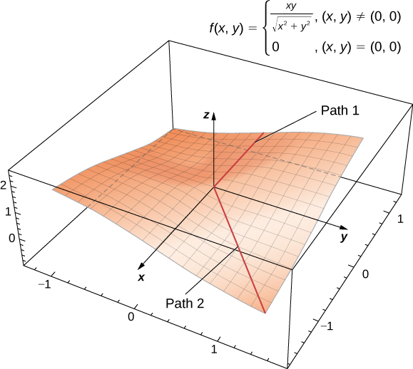
A tangent plane to a surface does not always exist at every point on the surface. Consider the piecewise function
f(x,y)={xy√x2+y2,(x,y)≠(0,0)0,(x,y)=(0,0).
The graph of this function follows.
Figure 13.4.3: Graph of a function that does not have a tangent plane at the origin. Dynamic figure powered by CalcPlot3D.
If either x=0 or y=0, then f(x,y)=0, so the value of the function does not change on either the x- or y-axis. Therefore, fx(x,0)=fy(0,y)=0, so as either x or y approach zero, these partial derivatives stay equal to zero. Substituting them into Equation gives z=0 as the equation of the tangent line. However, if we approach the origin from a different direction, we get a different story. For example, suppose we approach the origin along the line y=x. If we put y=x into the original function, it becomes
f(x,x)=x(x)√x2+(x)2=x2√2x2=|x|√2.
When x>0, the slope of this curve is equal to √2/2; when x<0, the slope of this curve is equal to −(√2/2). This presents a problem. In the definition of tangent plane, we presumed that all tangent lines through point P (in this case, the origin) lay in the same plane. This is clearly not the case here. When we study differentiable functions, we will see that this function is not differentiable at the origin.
Linear Approximations
Recall from Linear Approximations and Differentials that the formula for the linear approximation of a function f(x) at the point x=a is given by
y≈f(a)+f′(a)(x−a).
The diagram for the linear approximation of a function of one variable appears in the following graph.
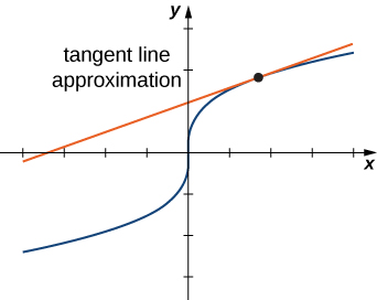
The tangent line can be used as an approximation to the function f(x) for values of x reasonably close to x=a. When working with a function of two variables, the tangent line is replaced by a tangent plane, but the approximation idea is much the same.
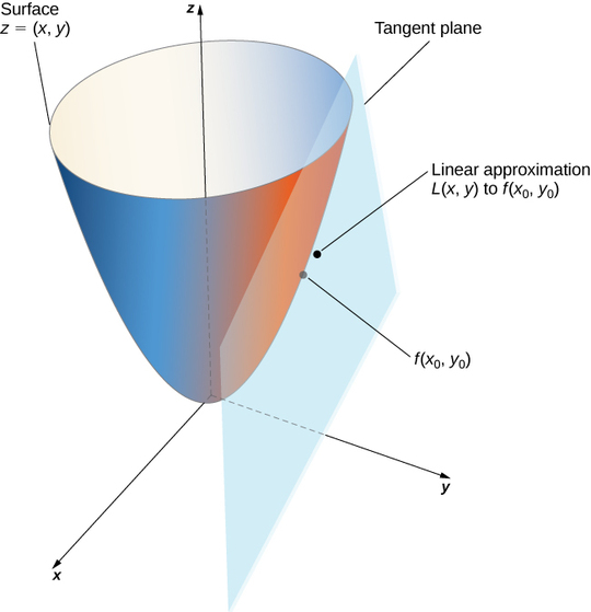
Given a function z=f(x,y) with continuous partial derivatives that exist at the point (x0,y0), the linear approximation of f at the point (x0,y0) is given by the equation
L(x,y)=f(x0,y0)+fx(x0,y0)(x−x0)+fy(x0,y0)(y−y0).
Notice that this equation also represents the tangent plane to the surface defined by z=f(x,y) at the point (x0,y0). The idea behind using a linear approximation is that, if there is a point (x0,y0) at which the precise value of f(x,y) is known, then for values of (x,y) reasonably close to (x0,y0), the linear approximation (i.e., tangent plane) yields a value that is also reasonably close to the exact value of f(x,y) (Figure 13.4.5). Furthermore the plane that is used to find the linear approximation is also the tangent plane to the surface at the point (x0,y0).
Given the function f(x,y)=√41−4x2−y2, approximate f(2.1,2.9) using point (2,3) for (x0,y0). What is the approximate value of f(2.1,2.9) to four decimal places?
Solution
To apply Equation ???, we first must calculate f(x0,y0),fx(x0,y0), and fy(x0,y0) using x0=2 and y0=3:
f(x0,y0)=f(2,3)=√41−4(2)2−(3)2=√41−16−9=√16=4fx(x,y)=−4x√41−4x2−y2 sofx(x0,y0)=−4(2)√41−4(2)2−(3)2=−2fy(x,y)=−y√41−4x2−y2 sofy(x0,y0)=−3√41−4(2)2−(3)2=−34.
Now we substitute these values into Equation ???:
L(x,y)=f(x0,y0)+fx(x0,y0)(x−x0)+fy(x0,y0)(y−y0)=4−2(x−2)−34(y−3)=414−2x−34y.
Last, we substitute x=2.1 and y=2.9 into L(x,y):
L(2.1,2.9)=414−2(2.1)−34(2.9)=10.25−4.2−2.175=3.875.
The approximate value of f(2.1,2.9) to four decimal places is
f(2.1,2.9)=√41−4(2.1)2−(2.9)2=√14.95≈3.8665,
which corresponds to a 0.2 error in approximation.
Given the function f(x,y)=e5−2x+3y, approximate f(4.1,0.9) using point (4,1) for (x0,y0). What is the approximate value of f(4.1,0.9) to four decimal places?
- Hint
-
First calculate f(x0,y0),fx(x0,y0), and fy(x0,y0) using x0=4 and y0=1, then use Equation ???.
- Answer
-
L(x,y)=6−2x+3y, so L(4.1,0.9)=6−2(4.1)+3(0.9)=0.5 f(4.1,0.9)=e5−2(4.1)+3(0.9)=e−0.5≈0.6065.
Differentiability
When working with a function y=f(x) of one variable, the function is said to be differentiable at a point x=a if f′(a) exists. Furthermore, if a function of one variable is differentiable at a point, the graph is “smooth” at that point (i.e., no corners exist) and a tangent line is well-defined at that point.
The idea behind differentiability of a function of two variables is connected to the idea of smoothness at that point. In this case, a surface is considered to be smooth at point P if a tangent plane to the surface exists at that point. If a function is differentiable at a point, then a tangent plane to the surface exists at that point. Recall the formula (Equation ???) for a tangent plane at a point (x0,y0) is given by
z=f(x0,y0)+fx(x0,y0)(x−x0)+fy(x0,y0)(y−y0)
For a tangent plane to exist at the point (x0,y0), the partial derivatives must therefore exist at that point. However, this is not a sufficient condition for smoothness, as was illustrated in Figure 13.4.3. In that case, the partial derivatives existed at the origin, but the function also had a corner on the graph at the origin.
A function f(x,y) is differentiable at a point P(x0,y0) if, for all points (x,y) in a δ disk around P, we can write
f(x,y)=f(x0,y0)+fx(x0,y0)(x−x0)+fy(x0,y0)(y−y0)+E(x,y),
where the error term E satisfies
lim(x,y)→(x0,y0)E(x,y)√(x−x0)2+(y−y0)2=0.
The last term in Equation ??? is referred to as the error term and it represents how closely the tangent plane comes to the surface in a small neighborhood (δ disk) of point P. For the function f to be differentiable at P, the function must be smooth—that is, the graph of f must be close to the tangent plane for points near P.
Show that the function f(x,y)=2x2−4y is differentiable at point (2,−3).
Solution
First, we calculate f(x0,y0),fx(x0,y0), and fy(x0,y0) using x0=2 and y0=−3, then we use Equation ???:
f(2,−3)=2(2)2−4(−3)=8+12=20fx(2,−3)=4(2)=8fy(2,−3)=−4.
Therefore m1=8 and m2=−4, and Equation ??? becomes
f(x,y)=f(2,−3)+fx(2,−3)(x−2)+fy(2,−3)(y+3)+E(x,y)2x2−4y=20+8(x−2)−4(y+3)+E(x,y)2x2−4y=20+8x−16−4y−12+E(x,y)2x2−4y=8x−4y−8+E(x,y)E(x,y)=2x2−8x+8.
Next, we calculate the limit in Equation ???:
lim(x,y)→(x0,y0)E(x,y)√(x−x0)2+(y−y0)2=lim(x,y)→(2,−3)2x2−8x+8√(x−2)2+(y+3)2=lim(x,y)→(2,−3)2(x2−4x+4)√(x−2)2+(y+3)2=lim(x,y)→(2,−3)2(x−2)2√(x−2)2+(y+3)2≤lim(x,y)→(2,−3)2((x−2)2+(y+3)2)√(x−2)2+(y+3)2=lim(x,y)→(2,−3)2√(x−2)2+(y+3)2=0.
Since E(x,y)≥0 for any value of x or y, the original limit must be equal to zero. Therefore, f(x,y)=2x2−4y is differentiable at point (2,−3).
Show that the function f(x,y)=3x−4y2 is differentiable at point (−1,2).
- Hint
-
First, calculate f(x0,y0),fx(x0,y0), and fy(x0,y0) using x0=−1 and y0=2, then use Equation ??? to find E(x,y).
Since you will find that E(x,y)≤0, show lim(x,y)→(x0,y0)|E(x,y)|√(x−x0)2+(y−y0)2=0
- Answer
-
f(−1,2)=−19,fx(−1,2)=3,fy(−1,2)=−16,E(x,y)=−4(y−2)2.lim(x,y)→(x0,y0)|E(x,y)|√(x−x0)2+(y−y0)2=lim(x,y)→(−1,2)|−4(y−2)2|√(x+1)2+(y−2)2=lim(x,y)→(−1,2)4(y−2)2√(x+1)2+(y−2)2≤lim(x,y)→(−1,2)4((x+1)2+(y−2)2)√(x+1)2+(y−2)2=lim(x,y)→(−1,2)4√(x+1)2+(y−2)2=0.
Since lim(x,y)→(x0,y0)|E(x,y)|√(x−x0)2+(y−y0)2=0, we know it's also true that
lim(x,y)→(x0,y0)E(x,y)√(x−x0)2+(y−y0)2=0
Therefore, f(x,y)=3x−4y2 is differentiable at point (−1,2).
This function from (Equation ???)
f(x,y)={xy√x2+y2,(x,y)≠(0,0)0,(x,y)=(0,0)
is not differentiable at the origin (Figure 13.4.3). We can see this by calculating the partial derivatives. This function appeared earlier in the section, where we showed that fx(0,0)=fy(0,0)=0. Substituting this information into Equations ??? and ??? using x0=0 and y0=0, we get
f(x,y)=f(0,0)+fx(0,0)(x−0)+fy(0,0)(y−0)+E(x,y)E(x,y)=xy√x2+y2.
Calculating
lim(x,y)→(x0,y0)E(x,y)√(x−x0)2+(y−y0)2
gives
lim(x,y)→(x0,y0)E(x,y)√(x−x0)2+(y−y0)2=lim(x,y)→(0,0)xy√x2+y2√x2+y2=lim(x,y)→(0,0)xyx2+y2.
Depending on the path taken toward the origin, this limit takes different values. Therefore, the limit does not exist and the function f is not differentiable at the origin as shown in the following figure.
Differentiability and continuity for functions of two or more variables are connected, the same as for functions of one variable. In fact, with some adjustments of notation, the basic theorem is the same.
Let z=f(x,y) be a function of two variables with (x0,y0) in the domain of f. If f(x,y) is differentiable at (x0,y0), then f(x,y) is continuous at (x0,y0).
Theorem 13.4.1 shows that if a function is differentiable at a point, then it is continuous there. However, if a function is continuous at a point, then it is not necessarily differentiable at that point. For example, the function discussed above (Equation ???)
f(x,y)={xy√x2+y2,(x,y)≠(0,0)0,(x,y)=(0,0)
is continuous at the origin, but it is not differentiable at the origin. This observation is also similar to the situation in single-variable calculus.
We can further explore the connection between continuity and differentiability at a point. This next theorem says that if the function and its partial derivatives are continuous at a point, the function is differentiable.
Let z=f(x,y) be a function of two variables with (x0,y0) in the domain of f. If f(x,y), fx(x,y), and fy(x,y) all exist in a neighborhood of (x0,y0) and are continuous at (x0,y0), then f(x,y) is differentiable there.
Recall that earlier we showed that the function in Equation ??? was not differentiable at the origin. Let’s calculate the partial derivatives fx and fy:
∂f∂x=y3(x2+y2)3/2
and
∂f∂y=x3(x2+y2)3/2.
The contrapositive of the preceding theorem states that if a function is not differentiable, then at least one of the hypotheses must be false. Let’s explore the condition that fx(0,0) must be continuous. For this to be true, it must be true that
lim(x,y)→(0,0)fx(x,y)=fx(0,0)
therefor
lim(x,y)→(0,0)fx(x,y)=lim(x,y)→(0,0)y3(x2+y2)3/2.
Let x=ky. Then
lim(x,y)→(0,0)y3(x2+y2)3/2=limy→0y3((ky)2+y2)3/2=limy→0y3(k2y2+y2)3/2=limy→0y3|y|3(k2+1)3/2=1(k2+1)3/2limy→0|y|y.
If y>0, then this expression equals 1/(k2+1)3/2; if y<0, then it equals −(1/(k2+1)3/2). In either case, the value depends on k, so the limit fails to exist.
Differentials
In Linear Approximations and Differentials we first studied the concept of differentials. The differential of y, written dy, is defined as f′(x)dx. The differential is used to approximate Δy=f(x+Δx)−f(x), where Δx=dx. Extending this idea to the linear approximation of a function of two variables at the point (x0,y0) yields the formula for the total differential for a function of two variables.
Let z=f(x,y) be a function of two variables with (x0,y0) in the domain of f, and let Δx and Δy be chosen so that (x0+Δx,y0+Δy) is also in the domain of f. If f is differentiable at the point (x0,y0), then the differentials dx and dy are defined as
dx=Δx
and
dy=Δy.
The differential dz, also called the total differential of z=f(x,y) at (x0,y0), is defined as
dz=fx(x0,y0)dx+fy(x0,y0)dy.
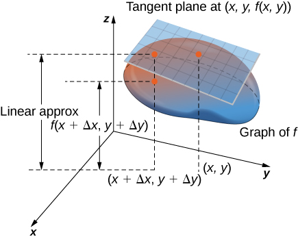
Notice that the symbol ∂ is not used to denote the total differential; rather, d appears in front of z. Now, let’s define Δz=f(x+Δx,y+Δy)−f(x,y). We use dz to approximate Δz, so
Δz≈dz=fx(x0,y0)dx+fy(x0,y0)dy.
Therefore, the differential is used to approximate the change in the function z=f(x0,y0) at the point (x0,y0) for given values of Δx and Δy. Since Δz=f(x+Δx,y+Δy)−f(x,y), this can be used further to approximate f(x+Δx,y+Δy):
f(x+Δx,y+Δy)=f(x,y)+Δz≈f(x,y)+fx(x0,y0)Δx+fy(x0,y0)Δy.
See the following figure.
One such application of this idea is to determine error propagation. For example, if we are manufacturing a gadget and are off by a certain amount in measuring a given quantity, the differential can be used to estimate the error in the total volume of the gadget.
Find the differential dz of the function f(x,y)=3x2−2xy+y2 and use it to approximate Δz at point (2,−3). Use Δx=0.1 and Δy=−0.05. What is the exact value of Δz?
Solution
First, we must calculate f(x0,y0),fx(x0,y0), and fy(x0,y0) using x0=2 and y0=−3:
f(x0,y0)=f(2,−3)=3(2)2−2(2)(−3)+(−3)2=12+12+9=33fx(x,y)=6x−2yfy(x,y)=−2x+2yfx(x0,y0)=fx(2,−3)=6(2)−2(−3)=12+6=18fy(x0,y0)=fy(2,−3)=−2(2)+2(−3)=−4−6=−10.
Then, we substitute these quantities into Equation ???:
dz=fx(x0,y0)dx+fy(x0,y0)dydz=18(0.1)−10(−0.05)=1.8+0.5=2.3.
This is the approximation to Δz=f(x0+Δx,y0+Δy)−f(x0,y0). The exact value of Δz is given by
Δz=f(x0+Δx,y0+Δy)−f(x0,y0)=f(2+0.1,−3−0.05)−f(2,−3)=f(2.1,−3.05)−f(2,−3)=2.3425.
Find the differential dz of the function f(x,y)=4y2+x2y−2xy and use it to approximate Δz at point (1,−1). Use Δx=0.03 and Δy=−0.02. What is the exact value of Δz?
- Hint
-
First, calculate fx(x0,y0) and fy(x0,y0) using x0=1 and y0=−1, then use Equation ???.
- Answer
-
dz=0.18
Δz=f(1.03,−1.02)−f(1,−1)=0.180682
Differentiability of a Function of Three Variables
All of the preceding results for differentiability of functions of two variables can be generalized to functions of three variables. First, the definition:
A function f(x,y,z) is differentiable at a point P(x0,y0,z0) if for all points (x,y,z) in a δ disk around P we can write
f(x,y)=f(x0,y0,z0)+fx(x0,y0,z0)(x−x0)+fy(x0,y0,z0)(y−y0)+fz(x0,y0,z0)(z−z0)+E(x,y,z),
where the error term E satisfies
lim(x,y,z)→(x0,y0,z0)E(x,y,z)√(x−x0)2+(y−y0)2+(z−z0)2=0.
If a function of three variables is differentiable at a point (x0,y0,z0), then it is continuous there. Furthermore, continuity of first partial derivatives at that point guarantees differentiability.
Key Concepts
- The analog of a tangent line to a curve is a tangent plane to a surface for functions of two variables.
- Tangent planes can be used to approximate values of functions near known values.
- A function is differentiable at a point if it is ”smooth” at that point (i.e., no corners or discontinuities exist at that point).
- The total differential can be used to approximate the change in a function z=f(x0,y0) at the point (x0,y0) for given values of Δx and Δy.
Key Equations
- Tangent plane
z=f(x0,y0)+fx(x0,y0)(x−x0)+fy(x0,y0)(y−y0)
- Linear approximation
L(x,y)=f(x0,y0)+fx(x0,y0)(x−x0)+fy(x0,y0)(y−y0)
- Total differential
dz=fx(x0,y0)dx+fy(x0,y0)dy.
- Differentiability (two variables)
f(x,y)=f(x0,y0)+fx(x0,y0)(x−x0)+fy(x0,y0)(y−y0)+E(x,y),
where the error term E satisfies
lim(x,y)→(x0,y0)E(x,y)√(x−x0)2+(y−y0)2=0.
- Differentiability (three variables)
f(x,y)=f(x0,y0,z0)+fx(x0,y0,z0)(x−x0)+fy(x0,y0,z0)(y−y0)+fz(x0,y0,z0)(z−z0)+E(x,y,z),
where the error term E satisfies
lim(x,y,z)→(x0,y0,z0)E(x,y,z)√(x−x0)2+(y−y0)2+(z−z0)2=0.
Glossary
- differentiable
-
a function f(x,y) is differentiable at (x0,y0) if f(x,y) can be expressed in the form f(x,y)=f(x0,y0)+fx(x0,y0)(x−x0)+fy(x0,y0)(y−y0)+E(x,y),
where the error term E(x,y) satisfies lim(x,y)→(x0,y0)E(x,y)√(x−x0)2+(y−y0)2=0
- linear approximation
- given a function f(x,y) and a tangent plane to the function at a point (x0,y0), we can approximate f(x,y) for points near (x0,y0) using the tangent plane formula
- tangent plane
- given a function f(x,y) that is differentiable at a point (x0,y0), the equation of the tangent plane to the surface z=f(x,y) is given by z=f(x0,y0)+fx(x0,y0)(x−x0)+fy(x0,y0)(y−y0)
- total differential
- the total differential of the function f(x,y) at (x0,y0) is given by the formula dz=fx(x0,y0)dx+fy(x0,y0)dy