Mathematics LibreTexts

Optimization of Functions of Several Variables

  • Page ID
    21131
  • \( \newcommand{\vecs}[1]{\overset { \scriptstyle \rightharpoonup} {\mathbf{#1}} } \)

    \( \newcommand{\vecd}[1]{\overset{-\!-\!\rightharpoonup}{\vphantom{a}\smash {#1}}} \)

    \( \newcommand{\id}{\mathrm{id}}\) \( \newcommand{\Span}{\mathrm{span}}\)

    ( \newcommand{\kernel}{\mathrm{null}\,}\) \( \newcommand{\range}{\mathrm{range}\,}\)

    \( \newcommand{\RealPart}{\mathrm{Re}}\) \( \newcommand{\ImaginaryPart}{\mathrm{Im}}\)

    \( \newcommand{\Argument}{\mathrm{Arg}}\) \( \newcommand{\norm}[1]{\| #1 \|}\)

    \( \newcommand{\inner}[2]{\langle #1, #2 \rangle}\)

    \( \newcommand{\Span}{\mathrm{span}}\)

    \( \newcommand{\id}{\mathrm{id}}\)

    \( \newcommand{\Span}{\mathrm{span}}\)

    \( \newcommand{\kernel}{\mathrm{null}\,}\)

    \( \newcommand{\range}{\mathrm{range}\,}\)

    \( \newcommand{\RealPart}{\mathrm{Re}}\)

    \( \newcommand{\ImaginaryPart}{\mathrm{Im}}\)

    \( \newcommand{\Argument}{\mathrm{Arg}}\)

    \( \newcommand{\norm}[1]{\| #1 \|}\)

    \( \newcommand{\inner}[2]{\langle #1, #2 \rangle}\)

    \( \newcommand{\Span}{\mathrm{span}}\) \( \newcommand{\AA}{\unicode[.8,0]{x212B}}\)

    \( \newcommand{\vectorA}[1]{\vec{#1}}      % arrow\)

    \( \newcommand{\vectorAt}[1]{\vec{\text{#1}}}      % arrow\)

    \( \newcommand{\vectorB}[1]{\overset { \scriptstyle \rightharpoonup} {\mathbf{#1}} } \)

    \( \newcommand{\vectorC}[1]{\textbf{#1}} \)

    \( \newcommand{\vectorD}[1]{\overrightarrow{#1}} \)

    \( \newcommand{\vectorDt}[1]{\overrightarrow{\text{#1}}} \)

    \( \newcommand{\vectE}[1]{\overset{-\!-\!\rightharpoonup}{\vphantom{a}\smash{\mathbf {#1}}}} \)

    \( \newcommand{\vecs}[1]{\overset { \scriptstyle \rightharpoonup} {\mathbf{#1}} } \)

    \( \newcommand{\vecd}[1]{\overset{-\!-\!\rightharpoonup}{\vphantom{a}\smash {#1}}} \)

    \(\newcommand{\avec}{\mathbf a}\) \(\newcommand{\bvec}{\mathbf b}\) \(\newcommand{\cvec}{\mathbf c}\) \(\newcommand{\dvec}{\mathbf d}\) \(\newcommand{\dtil}{\widetilde{\mathbf d}}\) \(\newcommand{\evec}{\mathbf e}\) \(\newcommand{\fvec}{\mathbf f}\) \(\newcommand{\nvec}{\mathbf n}\) \(\newcommand{\pvec}{\mathbf p}\) \(\newcommand{\qvec}{\mathbf q}\) \(\newcommand{\svec}{\mathbf s}\) \(\newcommand{\tvec}{\mathbf t}\) \(\newcommand{\uvec}{\mathbf u}\) \(\newcommand{\vvec}{\mathbf v}\) \(\newcommand{\wvec}{\mathbf w}\) \(\newcommand{\xvec}{\mathbf x}\) \(\newcommand{\yvec}{\mathbf y}\) \(\newcommand{\zvec}{\mathbf z}\) \(\newcommand{\rvec}{\mathbf r}\) \(\newcommand{\mvec}{\mathbf m}\) \(\newcommand{\zerovec}{\mathbf 0}\) \(\newcommand{\onevec}{\mathbf 1}\) \(\newcommand{\real}{\mathbb R}\) \(\newcommand{\twovec}[2]{\left[\begin{array}{r}#1 \\ #2 \end{array}\right]}\) \(\newcommand{\ctwovec}[2]{\left[\begin{array}{c}#1 \\ #2 \end{array}\right]}\) \(\newcommand{\threevec}[3]{\left[\begin{array}{r}#1 \\ #2 \\ #3 \end{array}\right]}\) \(\newcommand{\cthreevec}[3]{\left[\begin{array}{c}#1 \\ #2 \\ #3 \end{array}\right]}\) \(\newcommand{\fourvec}[4]{\left[\begin{array}{r}#1 \\ #2 \\ #3 \\ #4 \end{array}\right]}\) \(\newcommand{\cfourvec}[4]{\left[\begin{array}{c}#1 \\ #2 \\ #3 \\ #4 \end{array}\right]}\) \(\newcommand{\fivevec}[5]{\left[\begin{array}{r}#1 \\ #2 \\ #3 \\ #4 \\ #5 \\ \end{array}\right]}\) \(\newcommand{\cfivevec}[5]{\left[\begin{array}{c}#1 \\ #2 \\ #3 \\ #4 \\ #5 \\ \end{array}\right]}\) \(\newcommand{\mattwo}[4]{\left[\begin{array}{rr}#1 \amp #2 \\ #3 \amp #4 \\ \end{array}\right]}\) \(\newcommand{\laspan}[1]{\text{Span}\{#1\}}\) \(\newcommand{\bcal}{\cal B}\) \(\newcommand{\ccal}{\cal C}\) \(\newcommand{\scal}{\cal S}\) \(\newcommand{\wcal}{\cal W}\) \(\newcommand{\ecal}{\cal E}\) \(\newcommand{\coords}[2]{\left\{#1\right\}_{#2}}\) \(\newcommand{\gray}[1]{\color{gray}{#1}}\) \(\newcommand{\lgray}[1]{\color{lightgray}{#1}}\) \(\newcommand{\rank}{\operatorname{rank}}\) \(\newcommand{\row}{\text{Row}}\) \(\newcommand{\col}{\text{Col}}\) \(\renewcommand{\row}{\text{Row}}\) \(\newcommand{\nul}{\text{Nul}}\) \(\newcommand{\var}{\text{Var}}\) \(\newcommand{\corr}{\text{corr}}\) \(\newcommand{\len}[1]{\left|#1\right|}\) \(\newcommand{\bbar}{\overline{\bvec}}\) \(\newcommand{\bhat}{\widehat{\bvec}}\) \(\newcommand{\bperp}{\bvec^\perp}\) \(\newcommand{\xhat}{\widehat{\xvec}}\) \(\newcommand{\vhat}{\widehat{\vvec}}\) \(\newcommand{\uhat}{\widehat{\uvec}}\) \(\newcommand{\what}{\widehat{\wvec}}\) \(\newcommand{\Sighat}{\widehat{\Sigma}}\) \(\newcommand{\lt}{<}\) \(\newcommand{\gt}{>}\) \(\newcommand{\amp}{&}\) \(\definecolor{fillinmathshade}{gray}{0.9}\)

    One of the most useful applications for derivatives of a function of one variable is the determination of maximum and/or minimum values. This application is also important for functions of two or more variables, but as we have seen in earlier sections of this chapter, the introduction of more independent variables leads to more possible outcomes for the calculations. The main ideas of finding critical points and using derivative tests are still valid, but new wrinkles appear when assessing the results.

    Critical Points

    For functions of a single variable, we defined critical points as the values of the function when the derivative equals zero or does not exist. For functions of two or more variables, the concept is essentially the same, except for the fact that we are now working with partial derivatives.

    Definition: Critical Points

    Let \(z=f(x,y)\) be a function of two variables that is differentiable on an open set containing the point \((x_0,y_0)\). The point \((x_0,y_0)\) is called a critical point of a function of two variables \(f\) if one of the two following conditions holds:

    1. \(f_x(x_0,y_0)=f_y(x_0,y_0)=0\)
    2. Either \(f_x(x_0,y_0) \; \text{or} \; f_y(x_0,y_0)\) does not exist.

    Example \(\PageIndex{1}\): Finding Critical Points

    Find the critical points of each of the following functions:

    1. \(f(x,y)=\sqrt{4y^2−9x^2+24y+36x+36}\)
    2. \(g(x,y)=x^2+2xy−4y^2+4x−6y+4\)

    Solution:

    a. First, we calculate \(f_x(x,y) \; \text{and} \; f_y(x,y):\)

    \[\begin{align*} f_x(x,y)&=\dfrac{1}{2}(−18x+36)(4y^2−9x^2+24y+36x+36)^{−1/2} \\ &=\dfrac{−9x+18}{\sqrt{4y^2−9x^2+24y+36x+36}} \end{align*}\]

    \[\begin{align*} f_y(x,y)&=\dfrac{1}{2}(8y+24)(4y^2−9x^2+24y+36x+36)^{−1/2} \\ &=\dfrac{4y+12}{\sqrt{4y^2−9x^2+24y+36x+36}} \end{align*}.\]

    Next, we set each of these expressions equal to zero:

    \[\begin{align*} \dfrac{−9x+18}{\sqrt{4y^2−9x^2+24y+36x+36}}&=0 \\ \dfrac{4y+12}{\sqrt{4y^2−9x^2+24y+36x+36}}&=0. \end{align*}\]

    Then, multiply both sides of each equation by its denominator (to clear the denominators):

    \[\begin{align*} −9x+18&=0 \\ 4y+12&=0. \end{align*}\]

    Therefore, \(x=2\) and \(y=−3,\) so \((2,−3)\) is a critical point of \(f\).

    We must also check for the possibility that the denominator of each partial derivative can equal zero, thus causing the partial derivative not to exist. Since the denominator is the same in each partial derivative, we need only do this once:

    \[4y^2−9x^2+24y+36x+36=0. \nonumber\]

    This equation represents a hyperbola. We should also note that the domain of \(f\) consists of points satisfying the inequality

    \[4y^2−9x^2+24y+36x+36≥0. \nonumber\]

    Therefore, any points on the hyperbola are not only critical points, they are also on the boundary of the domain. To put the hyperbola in standard form, we use the method of completing the square:

    \[\begin{align*} 4y^2−9x^2+24y+36x+36&=0 \\ 4y^2−9x^2+24y+36x&=−36 \\ 4y^2+24y−9x^2+36x&=−36 \\ 4(y^2+6y)−9(x^2−4x)&=−36 \\ 4(y^2+6y+9)−9(x^2−4x+4)&=−36−36+36 \\ 4(y+3)^2−9(x−2)^2&=−36.\end{align*}\]

    Dividing both sides by \(−36\) puts the equation in standard form:

    \[\begin{align*} \dfrac{4(y+3)^2}{−36}−\dfrac{9(x−2)^2}{−36}&=1 \\ \dfrac{(x−2)^2}{4}−\dfrac{(y+3)^2}{9}&=1. \end{align*}\]

    Notice that point \((2,−3)\) is the center of the hyperbola.

    Thus, the critical points of the function \(f\) are \( (2, -3) \) and all points on the hyperbola, \(\dfrac{(x−2)^2}{4}−\dfrac{(y+3)^2}{9}=1\).


    b. First, we calculate \(g_x(x,y)\) and \(g_y(x,y)\):

    \[\begin{align*} g_x(x,y)&=2x+2y+4 \\ g_y(x,y)&=2x−8y−6. \end{align*}\]

    Next, we set each of these expressions equal to zero, which gives a system of equations in \(x\) and \(y\):

    \[\begin{align*} 2x+2y+4&=0 \\ 2x−8y−6&=0. \end{align*}\]

    Subtracting the second equation from the first gives \(10y+10=0\), so \(y=−1\). Substituting this into the first equation gives \(2x+2(−1)+4=0\), so \(x=−1\).

    Therefore \((−1,−1)\) is a critical point of \(g\). There are no points in \(\mathbb{R}^2\) that make either partial derivative not exist.

    Figure \(\PageIndex{1}\) shows the behavior of the surface at the critical point.

    imageedit_3_8654401108.png
    Figure \(\PageIndex{1}\): The function \(g(x,y)\) has a critical point at \((−1,−1,5)\).

    Exercise \(\PageIndex{1}\):

    Find the critical point of the function \(f(x,y)=x^3+2xy−2x−4y.\)

    Hint

    Calculate \(f_x(x,y)\) and \(f_y(x,y)\), then set them equal to zero.

    Answer

    The only critical point of \(f\) is \((2,−5)\).

    Determining Global and Local Extrema

    The main purpose for determining critical points is to locate relative maxima and minima, as in single-variable calculus. When working with a function of one variable, the definition of a local extremum involves finding an interval around the critical point such that the function value is either greater than or less than all the other function values in that interval. When working with a function of two or more variables, we work with an open disk around the point.

    Definition: Global and Local Extrema

    Let \(z=f(x,y)\) be a function of two variables that is defined and continuous on an open set containing the point \((x_0,y_0).\) Then \(f\) has a local maximum at \((x_0,y_0\)) if

    \[f(x_0,y_0)≥f(x,y)\]

    for all points \((x,y)\) within some disk centered at \((x_0,y_0)\). The number \(f(x_0,y_0)\) is called a local maximum value. If the preceding inequality holds for every point \((x,y)\) in the domain of \(f\), then \(f\) has a global maximum (also called an absolute maximum) at \((x_0,y_0).\)

    The function \(f\) has a local minimum at \((x_0,y_0)\) if

    \[f(x_0,y_0)≤f(x,y)\]

    for all points \((x,y)\) within some disk centered at \((x_0,y_0)\). The number \(f(x_0,y_0)\) is called a local minimum value. If the preceding inequality holds for every point \((x,y)\) in the domain of \(f\), then \(f\) has a global minimum (also called an absolute minimum) at \((x_0,y_0)\).

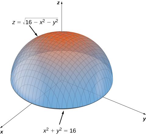
    If \(f(x_0,y_0)\) is either a local maximum or local minimum value, then it is called a local extremum (Figure \(\PageIndex{2}\)).

    imageedit_6_9229427091.png
    Figure \(\PageIndex{2}\): The graph of \(z=\sqrt{16−x^2−y^2}\) has a maximum value when \((x,y)=(0,0)\). It attains its minimum value at the boundary of its domain, which is the circle \(x^2+y^2=16.\)

    In Calculus 1, we showed that extrema of functions of one variable occur at critical points. The same is true for functions of more than one variable, as stated in the following theorem.

    Fermat’s Theorem for Functions of Two Variables

    Let \(z=f(x,y)\) be a function of two variables that is defined and continuous on an open set containing the point \((x_0,y_0)\). Suppose \(f_x\) and \(f_y\) each exists at \((x_0,y_0)\). If f has a local extremum at \((x_0,y_0)\), then \((x_0,y_0)\) is a critical point of \(f\).

    Consider the function \(f(x)=x^3.\) This function has a critical point at \(x=0\), since \(f'(0)=3(0)^2=0\). However, \(f\) does not have an extreme value at \(x=0\). Therefore, the existence of a critical value at \(x=x_0\) does not guarantee a local extremum at \(x=x_0\). The same is true for a function of two or more variables. One way this can happen is at a saddle point. An example of a saddle point appears in the following figure.

    Figure \(\PageIndex{3} \label{saddlefigure}\): Graph of the function \(z=x^2−y^2\). This graph has a saddle point at the origin.

    In this graph, the origin is a saddle point. This is because the first partial derivatives of f\((x,y)=x^2−y^2\) are both equal to zero at this point, but it is neither a maximum nor a minimum for the function. Furthermore the vertical trace corresponding to \(y=0\) is \(z=x^2\) (a parabola opening upward), but the vertical trace corresponding to \(x=0\) is \(z=−y^2\) (a parabola opening downward). Therefore, it is both a global maximum for one trace and a global minimum for another.

    Definition: Saddle Point

    Given the function \(z=f(x,y),\) the point \(\big(x_0,y_0,f(x_0,y_0)\big)\) is a saddle point if both \(f_x(x_0,y_0)=0\) and \(f_y(x_0,y_0)=0\), but \(f\) does not have a local extremum at \((x_0,y_0).\)

    Classifying Critical Points

    In order to develop a general method for classifying the behavior of a function of two variables at its critical points, we need to begin by classifying the behavior of quadratic polynomial functions of two variables at their critical points.

    To see why this will help us, consider that the quadratic approximation of a function of two variables (its 2nd-degree Taylor polynomial) shares the same first and second partials as the function it approximates at the chosen point of tangency (or center point). Since sharing the same second partials means the two surfaces will share the same concavity (or curvature) at the critical point, this causes these quadratic approximation surfaces to share the same behavior as the function \(z = f(x, y)\) that they approximate at the point of tangency. In other words, if the original function has a relative maximum at this point, so will the quadratic approximation. If the original function has a relative minimum at this point, so will the quadratic approximation, and if the original function has a saddle point at this point, so will the quadratic approximation.

    Now there are really three basic behaviors of a quadratic polynomial in two variables at a point where it has a critical point. It will fit one of the following three forms, often being a transformation of one of the following functions.

    1. A sum of two squared terms, like \(z = x^2 + y^2\), producing a paraboloid that opens up and has a relative (absolute) minimum at its vertex. See the plot on the left side of Figure \(\PageIndex{4}\).
    2. The negative of a sum of two squared terms, like \(z = -\left(x^2 + y^2\right)\), producing a paraboloid that opens down and has a relative (absolute) maximum at its vertex. See the plot on the right side of Figure \(\PageIndex{4}\).
    3. The difference of two squared terms, like \(z = f(x, y) = x^2 - y^2\) or \(z = f(x, y) = y^2 - x^2\), producing a saddle with a saddle point at its critical point. See Figure \(\PageIndex{3}\).

    Figure \(\PageIndex{4}\): \(z = x^2 + y^2\) has an absolute minimum of \(0\) at \( (0,0)\), while \(z = -(x^2 + y^2)\) has an absolute maximum of \(0\) at \( (0,0)\),

    Example \(\PageIndex{1}\): Classifying the critical points of a function

    Use completing the square to identify local extrema or saddle points of the following quadratic polynomial functions:

    1. \(f(x,y) = x^2 - 6x + y^2 + 10y + 20\)
    2. \(f(x,y) = 12 - 3x^2 - 6x - y^2 + 12y\)
    3. \(f(x,y) = x^2 + 8x - 2y^2 + 16y\)
    4. \(f(x,y) = x^2 + 6xy + y^2\)

    Solution

    a. To determine the critical points of this function, we start by setting the partials of \(f\) equal to \(0\). \[ \begin{align*} \text{Set}\quad f_x(x,y) &= 2x -6 = 0 & \implies x &= 3 \\ \text{and}\quad f_y(x,y) &= 2y + 10 = 0 & \implies y &= -5 \end{align*} \]We obtain a single critical point with coordinates \( (3, -5) \). Next we need to determine the behavior of the function \(f\) at this point.

    Completing the square, we get: \[\begin{align*} f(x,y) &= x^2 - 6x + y^2 + 10y + 20 \\ &= x^2 - 6x + 9 + y^2 + 10y + 25 + 20 - 9 - 25 \\ &= (x - 3)^2 + (y + 5)^2 - 14 \end{align*}\]Notice that this function is really just a translated version of \(z = x^2 + y^2\), so it is a paraboloid that opens up with its vertex (minimum point) at the critical point \( (3, -5) \). We can argue that it has an absolute minimum value of \(-14\) at the point \( (3, -5) \), since we are adding squared terms to \(-14\) and thus cannot get a value less than \(-14\) for any values of \(x\) and \(y\), while we do obtain this minimum value of \(-14\) at the vertex point \( (3, -5) \).

    b. Setting the partials of \(f\) equal to \(0\), we obtain: \[ \begin{align*} \text{Set}\quad f_x(x,y) &= -6x -6 = 0 & \implies x &= -1 \\ \text{and}\quad f_y(x,y) &= -2y + 12 = 0 & \implies y &= 6 \end{align*} \]We obtain a single critical point with coordinates \( (-1, 6) \). Next we need to determine the behavior of the function \(f\) at this point.

    To complete the square here, we first need to factor out the factors of the squared terms. Doing this and reordering the terms some gives us: \[\begin{align*} f(x,y) &= 12 - 3x^2 - 6x - y^2 + 12y\\ &= - 3\left(x^2 + 2x\quad\quad\right) - 1\left(y^2 - 12y \quad\quad\right) + 12 \\ &= -3\left(x^2 + 2x + 1\right) - 1\left(y^2 - 12y +36\right) + 12 +3+36\\ &= 51 - 3(x + 1)^2 - (y - 6)^2 \end{align*}\]Notice that this function is an elliptic paraboloid that opens down with its vertex (maximum point) at the critical point \( (-1, 6) \). We can argue that it has an absolute maximum value of \(51\) at the point \( (-1, 6) \), since we are subtracting squared terms from \(51\) and thus cannot get a value more than \(51\) for any values of \(x\) and \(y\), while we do obtain this minimum value of \(51\) at the vertex point \( (-1, 6) \).

    c. Setting the partials of \(f\) equal to \(0\), we obtain: \[ \begin{align*} \text{Set}\quad f_x(x,y) &= 2x + 8 = 0 & \implies x &= -4 \\ \text{and}\quad f_y(x,y) &= -4y + 16 = 0 & \implies y &= 4 \end{align*} \]This gives us a critical point with coordinates \( (-4, 4) \). To determine if \(f\) has a local extremum or saddle point at this point, we complete the square.

    Factoring out \(-2\) from the \(y\)-squared term gives us: \[\begin{align*} f(x,y) &= x^2 + 8x - 2y^2 + 16y \\ &= x^2 + 8x +16 - 2\left(y^2 - 8y + 16\right) - 16 + 32 \\ &= (x + 4)^2 - 2(y - 4)^2 +16\end{align*}\]Since one squared term is positive and one is negative, we see that this function has the form of \(z = x^2 - y^2\) and so it has a saddle point at its critical point. That is, \(f\) has a saddle point at \( (-4, 4, 16) \).

    d. Setting the partials of \(f\) equal to \(0\), we get: \[ \begin{align*} \text{Set}\quad f_x(x,y) &= 2x + 6y = 0 & \\ \text{and}\quad f_y(x,y) &= 6x + 2y = 0 & \implies y &= -3x \end{align*} \]Substituting \(-3x\) into the first equation for \(y\) gives us, \[\begin{align*}2x + 6(-3x) &= 0 \\ -16x &= 0 \\ x &= 0\end{align*}\]Since \(y = -3x\), we have \( y = -3(0) = 0\), so the critical point of \(f\) is \( (0,0) \). To determine the behavior of \(f\) at this critical point, we complete the square.

    \[\begin{align*} f(x,y) &= x^2 + 6xy + y^2 \\ &= (x^2 + 6xy + 9y^2) + y^2 - 9y^2 \\ &= (x + 3y)^2 - 8y^2 \end{align*}\]As this produces a difference of squares with one positive squared term and the other a negative squared term, we see that \(f\) takes a form similar to \(z = x^2 - y^2\) and will have a saddle point at \( (0, 0, 0) \).

    Now let's consider the quadratic approximation to a function \(z = f(x, y)\) centered at a critical point \( (x_0, y_0) \) of this function.

    \[Q(x, y) = f (x_0, y_0) + f_x(x_0, y_0) (x - x_0) + f_y(x_0, y_0) (y - y_0) + \frac{f_{xx}(x_0, y_0)}{2}(x-x_0)^2 + f_{xy}(x_0, y_0)(x-x_0)(y-y_0) + \frac{f_{yy}(x_0, y_0)}{2}(y-y_0)^2\]

    But, since the point \( (x_0, y_0) \), in this case, is a critical point of \(f\), we know that \(f_x(x_0, y_0) = 0\) and \(f_y(x_0, y_0) = 0\).

    This allows us to simplify \(Q(x, y)\) to just:

    \[Q(x, y) = f (x_0, y_0) + \frac{f_{xx}(x_0, y_0)}{2}(x-x_0)^2 + f_{xy}(x_0, y_0)(x-x_0)(y-y_0) + \frac{f_{yy}(x_0, y_0)}{2}(y-y_0)^2\]

    Now we need to complete the square on this quadratic polynomial in two variables to learn how we can classify the behavior of this function at this critical point. Remember that the original function will share the same behavior (max, min, saddle point) as this 2nd-degree Taylor polynomial at this critical point.

    To make this process easier, let's make some substitutions. Let's choose to let \(u = x - x_0\) and \(v = y - y_0\),

    and let \[\begin{align*} a &= \frac{f_{xx}(x_0, y_0)}{2}, \\ b &= f_{xy}(x_0, y_0), \\ c &= \frac{f_{yy}(x_0, y_0)}{2} \,\text{and} \\ d &= f (x_0, y_0) \end{align*}\]

    Then we need to complete the square on the polynomial: \[ Q(x,y) = au^2 +buv + cv^2 + d\]

    Completing the square:

    First we factor out the coefficient of \(u^2\): \[= a\left[ u^2 + \frac{b}{a}uv + \frac{c}{a}v^2\right] + d\]

    Next, we complete the square using the first two terms: \[= a\left[ \left(u^2 + \frac{b}{a}uv + \left(\frac{b}{2a}v\right)^2\right) + \frac{c}{a}v^2 - \left(\frac{b}{2a}v\right)^2 \right] + d\]

    Rewriting the perfect square trinomial as the square of a binomial and combining the \(v^2\) terms yields:

    \[\begin{align*} &= a\left[ \left(u+ \frac{b}{2a}v\right)^2 + \left(\frac{c}{a} - \frac{b^2}{4a^2}\right)v^2 \right] + d \\
    &= a\left[ \left(u+ \frac{b}{2a}v\right)^2 + \left(\frac{4ac}{4a^2} - \frac{b^2}{4a^2}\right)v^2 \right] + d \\
    &= a\left[ \left(u+ \frac{b}{2a}v\right)^2 + \left(\frac{4ac-b^2}{4a^2}\right)v^2 \right] + d \end{align*}\]

    Note that the shape of this function's graph depends on the sign of the coefficient of \(v^2\). And the sign of this coefficient is determined only by its numerator, as the denominator is always positive (being a perfect square). This expression, \(4ac-b^2\), is called the discriminant, as it helps us discriminate (tell the difference between) which behavior the function has at this critical point.

    If \(D = 4ac-b^2\gt 0\), then the two squared terms inside the brackets are both positive, and

    • if \(a = \frac{f_{xx}(x_0, y_0)}{2} \gt 0\), the function \(f\) opens upwards with a local minimum at the critical point \( (x_0, y_0) \). Note it would be similar to the form, \(z = x^2 + y^2\).
    • if \(a = \frac{f_{xx}(x_0, y_0)}{2} \lt 0\), the function \(f\) opens downwards with a local maximum at the critical point \( (x_0, y_0) \). Note it would be similar to the form, \(z = -\left(x^2 + y^2\right)\).

    If \(D = 4ac-b^2 \lt 0\), then either

    • the two squared terms inside the brackets have opposite signs (meaning \(f\) is concave up along a line parallel to the \(x\)-axis and concave down along a line parallel to the \(y\)-axis, or vice-versa) or
    • the \(b^2\) term, representing the square of the mixed partial \(f_{xy}(x_0, y_0)\), is larger than the positive product of the two 2nd-partials \(f_{xx}(x_0, y_0)\) and \(f_{yy}(x_0, y_0)\). This means that even if the surface is concave up in both \(x\)- and \(y\)-directions, or concave down in both \(x\)- and \(y\)-directions, a large mixed partial can offset these and cause the surface to have a saddle point at the point \((x_0, y_0)\).

    In either case, the quadratic polynomial will be in the form of \(z = x^2 - y^2\) or \(z = y^2 - x^2\) (i.e., it will be the difference of two squared terms), so we get a saddle point at the critical point \( (x_0, y_0) \).

    But if \(D = 4ac-b^2 = 0\), the quadratic polynomial reduces to \(Q(x,y) = a\left(u+ \frac{b}{2a}v\right)^2 + d\), whose graph is a parabolic cylinder, so the behavior of the function is not clear at the critical point \( (x_0, y_0) \).

    Now remembering the values of the constants \(a\), \(b\), and \(c\) from above, we see that: \[\begin{align*} D(x_0, y_0) &= 4\frac{f_{xx}(x_0, y_0)}{2}\frac{f_{yy}(x_0, y_0)}{2} - \big(f_{xy}(x_0, y_0)\big)^2 \\ &= f_{xx}(x_0, y_0)f_{yy}(x_0, y_0) - \big(f_{xy}(x_0, y_0)\big)^2 \end{align*}\]

    This formula is called the Second Partials Test, and it can be used to classify the behavior of any function at its critical points, as long as its second partials exist there and as long as the value of this discriminate is not zero.

    The Second Partials Test

    The second derivative test for a function of one variable provides a method for determining whether an extremum occurs at a critical point of a function. When extending this result to a function of two variables, an issue arises related to the fact that there are, in fact, four different second-order partial derivatives, although equality of mixed partials reduces this to three. The second partials test for a function of two variables, stated in the following theorem, uses a discriminant \(D\) that replaces \(f''(x_0)\) in the second derivative test for a function of one variable.

    second partials Test

    Let \(z=f(x,y)\) be a function of two variables for which the first- and second-order partial derivatives are continuous on some disk containing the point \((x_0,y_0)\). Suppose \(f_x(x_0,y_0)=0\) and \(f_y(x_0,y_0)=0.\) Define the quantity

    \[D=f_{xx}(x_0,y_0)f_{yy}(x_0,y_0)−\big(f_{xy}(x_0,y_0)\big)^2.\]

    Then:

    1. If \(D>0\) and \(f_{xx}(x_0,y_0)>0\), then \(f\) is concave up at this critical point, so \(f\) has a local minimum at \((x_0,y_0)\).
    2. If \(D>0\) and \(f_{xx}(x_0,y_0)<0\), then \(f\) is concave down at this critical point, so \(f\) has a local maximum at \((x_0,y_0)\).
    3. If \(D<0\), then \(f\) has a saddle point at \((x_0,y_0)\).
    4. If \(D=0\), then the test is inconclusive.

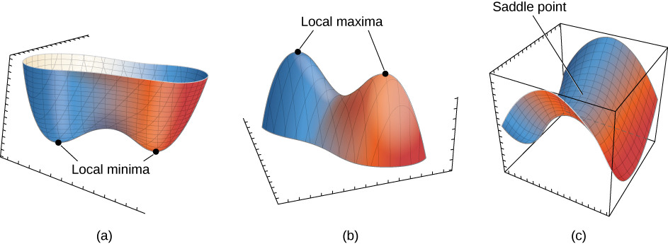
    See Figure \(\PageIndex{4}\).

    imageedit_9_5374076016.png
    Figure \(\PageIndex{4}\): The second partials test can often determine whether a function of two variables has a local minima (a), a local maxima (b), or a saddle point (c).

    To apply the second partials test, it is necessary that we first find the critical points of the function. There are several steps involved in the entire procedure, which are outlined in a problem-solving strategy.

    Problem-Solving Strategy: Using the second partials Test for Functions of Two Variables

    Let \(z=f(x,y)\) be a function of two variables for which the first- and second-order partial derivatives are continuous on some disk containing the point \((x_0,y_0).\)  To apply the second partials test to find local extrema, use the following steps:

    1. Determine the critical points \((x_0,y_0)\) of the function \(f\) where \(f_x(x_0,y_0)=f_y(x_0,y_0)=0.\)  If you find any critical points where at least one of the partial derivatives does not exist, you will need to find and justify extrema in another way, as you can't use the second partials test.
    2. Calculate the discriminant \(D=f_{xx}(x_0,y_0)f_{yy}(x_0,y_0)−\big(f_{xy}(x_0,y_0)\big)^2\) for each critical point of \(f\).
    3. Apply the four cases of the test to determine whether each critical point is a local maximum, local minimum, or saddle point, or whether the test is inconclusive.  If the test is inconclusive, you will need to analyze and classify the behavior at the critical point another way.

    Example \(\PageIndex{2}\): Using the second partials Test

    Find the critical points for each of the following functions, and use the second partials test to find any local extrema or saddle points.

    1. \(f(x,y)=4x^2+9y^2+8x−36y+24\)
    2. \(g(x,y)=\dfrac{1}{3}x^3+y^2+2xy−6x−3y+4\)

    Solution:

    a. Step 1 of the problem-solving strategy requires us to find the critical points of \(f\). To do this, we first calculate \(f_x(x,y)\) and \(f_y(x,y)\) and then set each of them equal to zero:

    \[\begin{align*} f_x(x,y)&=8x+8 \\ f_y(x,y)&=18y−36. \end{align*}\]

    Setting them equal to zero yields the system of equations

    \[\begin{align*} 8x+8&=0 \\ 18y−36&=0. \end{align*}\]

    The solution to this system is \(x=−1\) and \(y=2\). Therefore \((−1,2)\) is the only critical point of \(f\).

    Step 2 of the problem-solving strategy involves calculating \(D.\) To do this, we first calculate the second partial derivatives of \(f:\)

    \[\begin{align*} f_{xx}(x,y)&=8 \\ f_{xy}(x,y)&=0 \\ f_{yy}(x,y)&=18. \end{align*}\]

    Therefore, \(D(-1,2)=f_{xx}(−1,2)f_{yy}(−1,2)−\big(f_{xy}(−1,2)\big)^2=(8)(18)−(0)^2=144>0.\)

    Step 3 tells us to apply the four cases of the test to classify the function's behavior at this critical point.

    Since \(D>0\) and \(f_{xx}(−1,2)=8>0,\;f\) is concave up, so \(f\) has a local minimum of \(f(-1,2) = -16\) at \((−1,2)\), as shown in the following figure.  (Note that this corresponds to case 1 of the second partials test.)

    Figure \(\PageIndex{5}\): The function \(f(x,y)\) has a local minimum at \((−1,2,−16).\) Note the scale on the \(y\)-axis in this plot is in thousands.

    b. For step 1, we first calculate \(g_x(x,y)\) and \(g_y(x,y)\), then set each of them equal to zero:

    \[\begin{align*} g_x(x,y)&=x^2+2y−6 \\ g_y(x,y)&=2y+2x−3. \end{align*}\]

    Setting them equal to zero yields the system of equations

    \[\begin{align*} x^2+2y−6&=0 \\ 2y+2x−3&=0. \end{align*}\]

    To solve this system, first solve the second equation for \(y\). This gives \(y=\dfrac{3−2x}{2}\). Substituting this into the first equation gives

    \[\begin{align*} x^2+3−2x−6&=0 \\ x^2−2x−3&=0 \\ (x−3)(x+1)&=0. \end{align*}\]

    Therefore, \(x=−1\) or \(x=3\). Substituting these values into the equation \(y=\dfrac{3−2x}{2}\) yields the critical points \(\left(−1,\frac{5}{2}\right)\) and \(\left(3,−\frac{3}{2}\right)\).

    Step 2 involves calculating the second partial derivatives of \(g\):

    \[\begin{align*} g_{xx}(x,y)&=2x \\ g_{xy}(x,y)&=2\\ g_{yy}(x,y)&=2. \end{align*}\]

    Next, we substitute each critical point into the discriminant formula:

    \[\begin{align*} D\left(−1,\tfrac{5}{2}\right)&=(2(−1))(2)−(2)^2=−4−4=−8 \\ D\left(3,−\tfrac{3}{2}\right)&=(2(3))(2)−(2)^2=12−4=8. \end{align*}\]

    In step 3, we use the second partials test to classify the behavior of the function at each of its critical points.

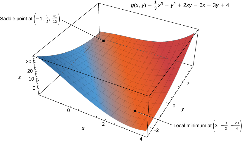
    At point \(\left(−1,\frac{5}{2}\right)\), we see that \(D\left(−1,\tfrac{5}{2}\right)=-8<0\) (case 3 of the test), which means that \(f\) has a saddle point at the point \(\left(−1,\frac{5}{2}\right)\).  The coordinates of this saddle point are \(\left(−1,\frac{5}{2}, \frac{41}{12}\right)\).

    Applying the theorem to point \(\left(3,−\frac{3}{2}\right)\) leads to case \(1\).  That is, since \(D\left(3,-\tfrac{3}{2}\right)=8>0\) and \(g_{xx}\left(3,-\tfrac{3}{2}\right)=2(3)=6>0\), we know that \(g\) is concave up at this critical point, so \(g\) has a local minimum of \(-\frac{29}{4}\) at the point \(\left(3,−\frac{3}{2}\right)\), as shown in the following figure.

    imageedit_12_6948063962.png
    Figure \(\PageIndex{6}\): The function \(g(x,y)\) has a local minimum and a saddle point.

    Note:  Sometimes it can be helpful to find a general formula for \(D\).  For example, here we could have used the following formula:

    \[\begin{align*} D(x_0, y_0) &=g_{xx}(x_0,y_0)g_{yy}(x_0,y_0)−\big(g_{xy}(x_0,y_0)\big)^2 \\ &=(2x_0)(2)−2^2\\ &=4x_0−4.\end{align*}\]

    Then we would have:

    \[\begin{align*} D\left(−1,\tfrac{5}{2}\right)&=4(-1)-4=−4−4=−8 \\ D\left(3,−\tfrac{3}{2}\right)&=4(3)-4=12−4=8. \end{align*}\]

    Note that the final values of the discriminant at each critical point are the same.

    Exercise \(\PageIndex{2}\)

    Use the second partials to find the local extrema of the function

    \[ f(x,y)=x^3+2xy−6x−4y^2. \nonumber\]

    Hint

    Follow the problem-solving strategy for applying the second partials test.

    Answer

    \(\left(\frac{4}{3},\frac{1}{3}\right)\) is a saddle point, \(\left(−\frac{3}{2},−\frac{3}{8}\right)\) is a local maximum. 


    Key Concepts

    • A critical point of the function \(f(x,y)\) is any point \((x_0,y_0)\) where either \(f_x(x_0,y_0)=f_y(x_0,y_0)=0\), or at least one of \(f_x(x_0,y_0)\) and \(f_y(x_0,y_0)\) do not exist.
    • A saddle point is a point \((x_0,y_0)\) where \(f_x(x_0,y_0)=f_y(x_0,y_0)=0\), but \((x_0,y_0)\) is neither a maximum nor a minimum at that point.
    • To find extrema of functions of two variables, first find the critical points, then calculate the discriminant and apply the second partials test.

    Key Equations

    • Discriminant

    \(D=f_{xx}(x_0,y_0)f_{yy}(x_0,y_0)−(f_{xy}(x_0,y_0))^2\)

    Glossary

    critical point of a function of two variables

    the point \((x_0,y_0)\) is called a critical point of \(f(x,y)\) if one of the two following conditions holds:

    1. \(f_x(x_0,y_0)=f_y(x_0,y_0)=0\)

    2. At least one of \(f_x(x_0,y_0)\) and \(f_y(x_0,y_0)\) do not exist

    discriminant
    the discriminant of the function \(f(x,y)\) is given by the formula \(D=f_{xx}(x_0,y_0)f_{yy}(x_0,y_0)−(f_{xy}(x_0,y_0))^2\)
    saddle point
    given the function \(z=f(x,y),\) the point \((x_0,y_0,f(x_0,y_0))\) is a saddle point if both \(f_x(x_0,y_0)=0\) and \(f_y(x_0,y_0)=0\), but \(f\) does not have a local extremum at \((x_0,y_0)\)

    Contributors

    • Gilbert Strang (MIT) and Edwin “Jed” Herman (Harvey Mudd) with many contributing authors. This content by OpenStax is licensed with a CC-BY-SA-NC 4.0 license. Download for free at http://cnx.org.

    • Paul Seeburger (Monroe Community College) edited and adapted this section extensively.
      Paul also wrote the entire subsection titled Classifying Critical Points.

    This page titled Optimization of Functions of Several Variables is shared under a CC BY-NC-SA license and was authored, remixed, and/or curated by OpenStax.