7.6: Putting It All Together

Learning Objectives

Students will be able to:

• Apply both a linear and an exponential regression to a single set of data
• Determine if a linear or exponential model is the better fit for the data
• Construct and use a model to make predictions based on the data

in order to apply mathematical modeling to solve real-world applications.

Using Models to Make Predictions

So far, we have explored both linear and exponential models for a given set of data. Our goal is to now take a given set of data and decide which is the better model to use, and ultimately to use the model to make a prediction of an output for a given input.

As a reminder, a scatter plot can be used to show the relationship (or correlation) between two related values: the input and the output variables. In this section, we shall create a scatter plot for a given set of data, and then use technology to determine a model that will allow us to make predictions.

One of the objectives in creating a model is to make predictions about values we have not yet measured by finding the mathematical relationship between the input and the output variables, and relate this to our theoretical understanding. In so doing we derive a mathematical relationship where y is a function of x.

\[y=\text{function of x} \\ or \\ y=f(x)\]

In this statement y is the output variable and plotted on the vertical axis and x is the input variable and plotted on the horizontal axis. Empirical data is collected through experimentation where x is changed and y is measured, with each data point being represented on a graph with the values (x,y). We have looked at linear and exponential functions so far, and the end of this chapter also discusses quadratic functions as another possible model.

\[\begin{align} y &=mx+b && \text{(linear function)} \\ y &= ab^{x} && \text{(exponential function)} \\ y &= ax^2+bx+c && \text{(quadratic function)} \end{align}\]

Each of the above equations has two variables (x,y) and two constants (m,b) or (a,b) except for the quadratic function which has three constants (a,b,c) and you should already know how to calculate the constants m(slope) and b (y-intercept) for a straight line from earlier in this chapter.

Our goals are three fold:

1. Use desmos to create a scatter plot of the given data.
2. Apply a linear and an exponential model and see which fits the data better.
3. Make a prediction of the value of an output by substituting the input into the better model.

In order to determine the better model, we need to pay attention to the value of r² that desmos gives us, which is the square of the correlation coefficient (r) mentioned in precious sections. When r²=1 the equation perfectly predicts the output variable and the data follows the equation exactly. When r²=0, the equation provides no correlation between the input and output variable. The closer r² is to 1, the more likely the model will provide accurate predictions, but it's also important to also look at the graph of the models and see if they reasonably fit the scatter plots. Do not blindly make predictions based on the value of r². You must always look at the phenomena you are studying to check for any predictions that are not physically possible. For example, if your input variable is the size of a rock, and your output variable is the weight of a rock, any model that predicts a negative weight for a given size wouldn't be reasonable.

Lets look at some data and fit it to the two different models we have explored in this chapter.

Example \(\PageIndex{1}\)

Table \(\PageIndex{1}\) shows a recent graduate’s credit card balance each month after graduation.

Table \(\PageIndex{1}\)

Month	1	2	3	4	5	6	7	8
Debt ($)	620.00	761.88	899.80	1039.93	1270.63	1589.04	1851.31	2154.92

1. Use a linear regression to fit a model to these data.

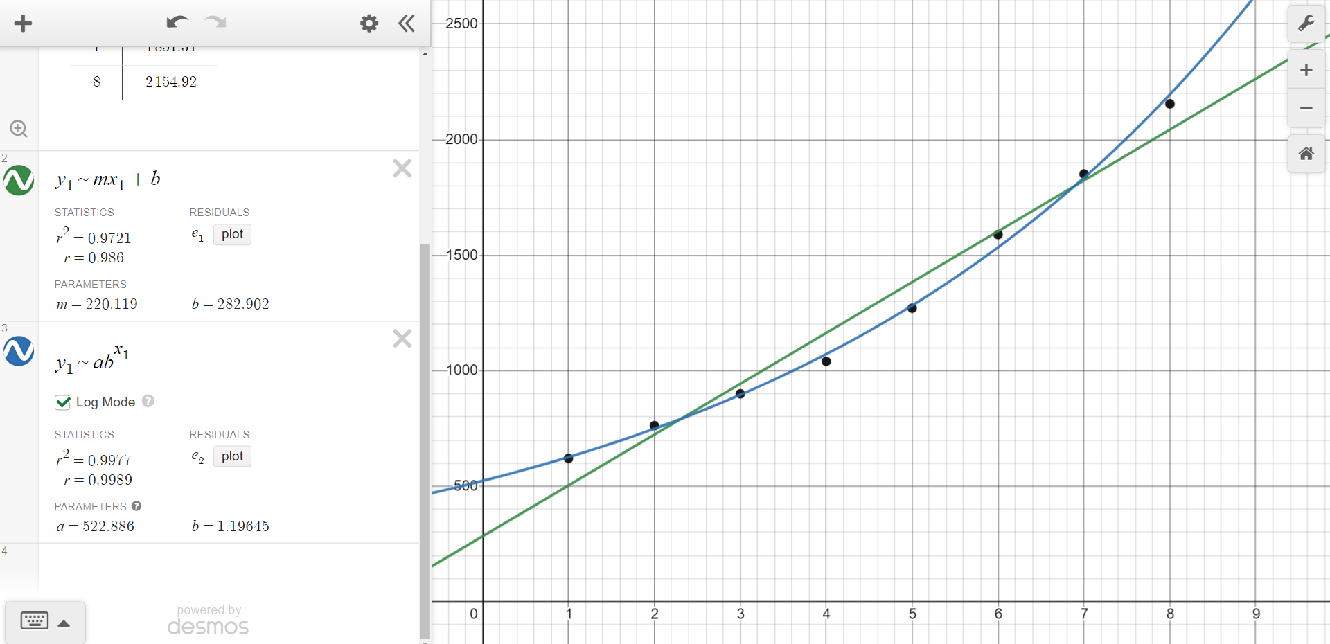
We will use desmos to recreate the table which will automatically generate a scatter plot. Then, following the same steps from the section on linear models, we type "y₁ ~ mx₁ + b" and desmos gives us "m = 220.119" and "b = 282.902". We are also given r² = 0.9721. This means the complete model is:

y = 220.11 x + 282.902

2. Use an exponential regression to fit a model to these data.

Using the same table already created in desmos from the previous step, we add the exponential model by typing "y₁ ~ ab^x₁" and desmos gives us "a = 522.886" and "b = 1.19645". We are also given r² = 0.9977. Please remember to click the box "Log Mode" to ensure you get the same results. This means the complete model is:

y= 522.886(1.19645^x)

3. Which model appears to fit the data better?

Looking at the values of r², it seems the exponential model is better. This is confirmed by visually looking at the models compared to the actual scatter plot. The figure below is what you should see on desmos.

4. Using the better model, make a prediction of the graduate’s credit card debt one year after graduating.

We will use the exponential model to make this prediction. Make sure to plug in 12 months and not 1 year since the original data is given in terms of months! We get the following:

y = 522.886(1.19645^x) = 522.886(1.19645¹²) = 4499.38

The graduate's credit card debt will be approximately $4,499.38 after one year. Had you used the linear model, you would have calculated a much different prediction of $2,924.33.

You can find this problem on desmos by clicking https://www.desmos.com/calculator/cx8igorint.