1.4: Types of Data

Not all data are the same. Next, we will discuss the different ways to classify statistical data.

A statistical variable is a characteristic that varies from one object to another. For example, age, major, GPA, and the desired grade are not the same for all students therefore each one of them is a statistical variable. The values of a variable for one or more people or things yield data. Here is an example of data collected from 3 students.

Table \(\PageIndex{1.1}\): An example of data collected from 3 students showing their age, major, GPA, and desired grade.

Age	Major	GPA	Desired Grade
19	Psychology	3.5	B
24	Criminal Justice	3.8	A
21	Nursing	3.6	A

Most variables and data can be put into the following categories: qualitative and quantitative.

Qualitative data consist of names and labels describing the attributes of a population such as hair color, blood type, ethnic group, the car a person drives, and the street a person lives on. Qualitative data are generally described by words or letters. For instance, hair color might be black, dark brown, light brown, blonde, gray, or red. Blood type might be AB+, O-, or B+.

Quantitative data consist of numbers that are the result of counting or measuring attributes of a population such as the amount of money, pulse rate, weight, number of people living in your town, and number of students who take statistics.

While numbers usually mean quantities, in general, not every number represents a quantity. For example, ZIP codes do not mean quantities therefore they are qualitative rather than quantitative type. Also, phone numbers, student IDs don’t mean quantities and since they are unique for each subject, they are called identifiers.

Qualitative data can be further classified as either ordinal or categorical. Ordinal data have a natural ordering, such as the letter grades, clothing size, and Likert scales. Qualitative data without a natural order is called categorical. For example, colors and college majors. There is also a special type of categorical data called binary when there are only two possible answer to a question such as yes/no or agree/disagree.

Quantitative data can be further classified as either discrete or continuous. All possible values of discrete data can be listed, while all possible values of continuous data form a continuous interval. For example: quantities, weights (rounded to pounds), ages (in years) are some examples of discrete type. Note that discrete data doesn't mean that the list is finite. On the other hand, the exact incomes, weights or heights, and time are some examples of continuous type.

Here is an example of different types of data collected from the same set of shows:

Table \(\PageIndex{1.2}\): An example of different types of data collected from the same set of shows

Rank	Show Title	Network	Viewers (millions)
1	CSI	CBS	19.3
2	NCIS	CBS	18.0
3	Dancing with Stars	ABC	17.8
4	Desperate Housewives	ABC	15.5
5	The Mentalist	CBS	14.9

The rank is discrete type, show title is the identifier, network is categorical, and number of millions of viewers is continuous.

Which type of data is more "complex"? From the least "complex" and most “boring” on the left to the most "complex" and “interesting” on the right, we can organize the data types in the following way:

Figure \(\PageIndex{1.3}\): The tree diagram showing the 4 types of data: categorical, ordinal, discrete, and continuous (from left to right).

Note that everything we can do with a less complex data type we would also be able to do with the more complex type of data. That is, we can do with discrete data everything that we can do with categorical data and some more!

Another way to classify the data is by the type of math operations that can be applied to the elements of the dataset. As a result, we have four levels of measurements: nominal, ordinal, interval, and ratio:

Figure \(\PageIndex{1.4}\): The tree diagram showing the 4 levels of measurements: nominal, ordinal, ratio, and interval (from left to right).

The nominal level is when the data cannot be arranged in any ordering scheme. For example: yes/no/undecided, political party affiliation.

The ordinal level is when the data can be arranged in some order but differences between data values either cannot be determined or are meaningless. For example: grades, ranks.

The interval level is when the data can be arranged in some order, for which the differences between data values are meaningful but there is no natural zero. For example: temperature, years.

The ratio level is when the data can be arranged in some order, for which the differences between data values are meaningful, and there is a natural zero that represents the absence of the quantity. For example: distances, prices.

Note that the first classification addresses what the data looks like and the latter classification addresses what can be done with the data mathematically. We can match the two classifications in the following way:

Figure \(\PageIndex{5}\): A diagram showing how the different levels of measurements align with different types of data.

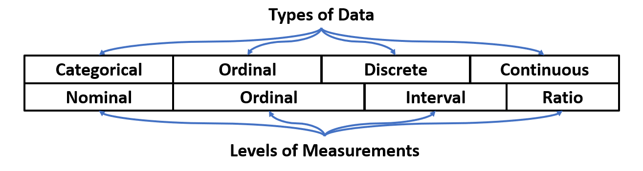
Also note that the framework of distinguishing levels of measurement originated in psychology and is widely criticized by scholars in other disciplines!