
7.2: Standard Types of Continuous Random Variables

( \newcommand{\kernel}{\mathrm{null}\,}\)
Section 1: Uniform Random Variable

Next, we will consider one of the standard continuous random variables called uniform and how to work with it.
A uniform probability density curve with parameters a and b is a horizontal line y=1b−a from x=a to x=b.

A random variable with a uniform probability density curve is called a uniform random variable with parameters a and b. We adopt the following notation to denote a uniform random variable with parameters a and b:
X∼U(a,b)
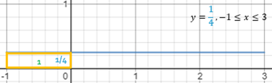
If X∼U(−1,3) is a uniform random variable with parameters −1 and 3 then its probability density curve will look like a horizontal line spanning from −1 to 3.

Easy to see that the graph satisfies the criteria for a probability density curve as it is above the x-axis and its area is the area of a rectangle with the base 4 and the height 14 which can be found using the formula for the area of a rectangle and is equal to 1.
Let’s find the probability of X=2. As we previously discussed, the probability of a continuous random variable being equal to a single value is equal to P(X=2)=0.

To find the probability that X is less than 2 we will look for the area under the curve between −1 and 2. This region is a rectangle with the base 3 and the height 14. The area can be found using the formula for the area of a rectangle and is equal to P(X<2)=0.75 or 75%.

To find the probability that X is less than 0 we will look for the area under the curve between −1 and 0. This region is a rectangle with the base 1 and the height 14. The area can be found using the formula for the area of a rectangle and is equal to P(−1<X<0)=0.25 or 25%.
To find the probability that X is between 0 and 2 we will look for the area under the curve between 0 and 2. This region is a rectangle with the base 2 and the height 14. The area can be found using the formula for the area of a rectangle and is equal to P(0<X<2)=0.5 or 50%. Alternatively, we could have used the subdivision rule to compute the same probability as the difference between the probability of X being less than 2 and the probability of X being less than 0 both of which we already computed previously, so the answer is again 50%.

To find the probability that X is greater than 2 we will look for the area under the curve between 2 and 3. This region is a rectangle with the base 1 and the height 14. The area can be found using the formula for the area of a rectangle and is equal to P(X>2)=0.25 or 25%. Alternatively, we could have used the complementary rule to compute the same probability as the complement of the probability of X being less than 2 which we already computed previously, so the answer is again 25%.

In general, for X∼U(a,b) and any c, d such that a<c<d<b:
P(c<X<d)=d−cb−a
P(X<d)=d−ab−a
P(X>c)=b−cb−a
Also,
μX=a+b2
σX=b−a√12
For example, for X∼U(−1,3):
P(0<X<2)=2−03−(−1)=24=0.50
P(X<0)=0−(−1)3−(−1)=14=0.25
P(X>2)=3−23−(−1)=14=0.25
Also,
μX=−1+32=2
σX=3−(−1)√12=1.15
A city metro train runs every 15 minutes.
- Find the probability that the waiting time is:
- less than 8 minutes;
- more than 3 minutes;
- between 3 and 7 minutes.
- Compute the following:
- the expected waiting time;
- the standard deviation of waiting time.
Solution
Waiting time is frequently estimated by a uniform random variable. Let X be the waiting time of a randomly selected passenger then it can be assumed uniform with parameters 0 and 15, i.e.:
X∼U(0,15)
Using the formulas we can compute all the quantities.
- Find the probability that the waiting time is:
- less than 8 minutes: P(X<8)=8−0)15−0=815=0.53
- more than 3 minutes: P(X>3)=15−315−0=1215=0.80
- between 3 and 7 minutes: P(3<X<7)=7−315−0=415=0.27
- Compute the following:
- the expected value of X: μX=0+152=7.5
- the standard deviation of X: σX=15−0√12=4.33
Section 2: Standard Normal Variable

The standard normal density curve is a bell-shaped curve that satisfies the following properties:
- Has the peak at 0 and symmetric about 0.
- Extends indefinitely in both directions, approaching but never touching the horizontal axis.
- The Empirical rule holds that is:
- ~68% of the area under the curve is between -1 and +1
- ~95% of the area under the curve is between -2 and +2
- ~99.7% of the area under the curve is between -3 and +3
The description of the curve should sound familiar as we have seen it before!

We define the standard normal random variable as a random variable with the standard normal probability density curve. We denote the standard normal random variable as
Z∼N(0,1)
Let’s make sure we understand the properties of the standard normal probability density curve and use the empirical rules to find some probabilities.
- To find the probability that X is less than 0 we will look for the area under the curve to the left of 0. This region’s area can be found by adding the areas of included regions together to get P(X<0)=0.50 or 50%.
- To find the probability that X is between −1 and 1 we will look for the area under the curve between −1 and 1. This region’s area can be found by adding the areas of included regions together to get P(−1<X<1)=0.68 or 68%.
- To find the probability that X is between 0 and 2 we will look for the area under the curve between 0 and 2. This region’s area can be found by adding the areas of included regions together to get P(0<X<2)=0.475 or 47.5%.
- To find the probability that X is between −1 and 2 we will look for the area under the curve between −1 and 2. This region’s area can be found by adding the areas of included regions together to get P(−1<X<2)=0.815 or 81.5%.
- To find the probability that X is greater than 1 we will look for the area under the curve to the right of 1. This region’s area can be found by adding the areas of included regions together to get P(X>1)=0.16 or 16%.
- To find the probability that X is less than −2 we will look for the area under the curve to the left of −2. This region’s area can be found by adding the areas of included regions together to get P(X<−2)=0.025 or 2.5%.
- To find the probability that X is greater than 4 we will look for the area under the curve to the right of 4. This region’s area is essentially equal to 0 so the probability is nearly 0%, that is P(X>4)=0.
To find the probability that X is less than 1.23 we will look for the area under the curve to the left of 1.23. While it is clear what this region’s area looks like it cannot be found by using the empirical rule.
So how do we find the probabilities that involve values that are not covered by the Empirical rule such as P(Z<1.23), P(Z>1.23), P(0<Z<1.23). The good news is that the latter two probabilities can be related to the first one by using the complementary rule and the subdivision rule:
P(Z>1.23)=1−P(Z<1.23)
P(0<Z<1.23)=P(Z<1.23)−0.5
But how do we find the probability P(Z<1.23)? Luckily all such probabilities have been computed and put together in the form of a table (part 1, part 2) that looks like this!

To find the probability that Z is less than 1.23 we split the number 1.23 into 1.2 and 0.03 then find the row corresponding to 1.2 and the column corresponding to 0.03. In the intersection, we find the desired probability, so the probability is P(Z<1.23)=0.8907 or 89.07%.
Now that we found the probability P(Z<1.23), we can find the other probabilities using the complementary rule and the subdivision rule:
- P(Z<1.23)=0.8907
- P(Z>1.23)=1−P(Z<1.23)=1−0.8907=0.1093
- P(0<Z<1.23)=P(Z<1.23)−0.5=0.8907−0.5=0.3907
Let’s practice using the table!
To find the probability that Z is less than 0.71, we split the number 0.71 into 0.7 and 0.01, find the row corresponding to 0.7, find the column corresponding to 0.01. In the intersection, we find the desired probability, so the probability is P(Z<0.71)=0.7611 or 76.11%. Also,
- P(Z<0.71)=0.7611
- P(Z>0.71)=1−P(Z<0.71)=1−0.7611=0.2389
- P(0<Z<0.71)=P(Z<0.71)−0.5=0.7611−0.5=0.2611
- P(0.71<Z<1.23)=P(Z<1.23)−P(Z<0.71)=0.8907−0.7611=0.1296
Example: To find the probability that Z is less than −1.02, we split the number −1.02 into −1.0 and −0.02, find the row corresponding to −1.0, find the column corresponding to −0.02. In the intersection, we find the desired probability, so the probability is P(Z<−1.02)=0.1539 or 15.39%. Also,
- P(Z<−1.02)=0.1539
- P(Z>−1.02)=1−P(Z<−1.02)=1−0.1539=0.8461
To find the probability that Z is less than −0.47, we split the number −0.47 into −0.4 and −0.07, find the row corresponding to −0.4, find the column corresponding to −0.07. In the intersection, we find the desired probability, so the probability is P(Z<−0.47)=0.3192 or 31.92%. Also,
- P(Z<−0.47)=0.3192
- P(Z>−0.47)=1−P(Z<−0.47)=1−0.3192=0.6808
- P(−1.02<Z<−0.47)=P(Z<−0.47)−P(Z<−1.02)=0.3192−0.1539=0.1653
Section 3: α-notation

Consider a random variable X and its probability density curve. A value the area to the right of which is equal to alpha is called xα.
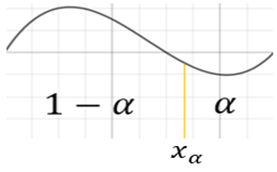
This fact can be expressed as the following probability statement:
P(X>xα)=α
As a result, the area to the left of xα is by the complementary rule must be 1−α. This fact can be expressed as the following probability statement:
P(X<xα)=1−α
For a continuous random variable X, the value the area to the right of which is equal to 0.3 is called x0.3.

This fact can be expressed as the following probability statement:
P(X>x0.3)=0.3
As a result, the area to the left of X is by the complementary rule must be 1−0.3=0.7. This fact can be expressed as the following probability statement:
P(X<x0.3)=0.7
Consider a uniform random variable with parameters −1 and 3, i.e., X∼U(−1,3). The value the area to the right of which is equal to 0.25 is called x0.25. In this case, we happened to know that x0.25=2.

This fact can be expressed in two ways:
P(X<x0.25)=0.75 and P(X>x0.25)=0.25
Consider a uniform random variable with parameters −1 and 3, i.e., X∼U(−1,3). The value the area to the left of which is equal to 0.6 is called x0.4. In this case, we happened to know that x0.40=1.4.

This fact can be expressed in two ways:
P(X<x0.4)=0.6 and P(X>x0.4)=0.4
In general, for a uniform random variable with parameters a and b, to find xα means to find the value the area to the right of which is α and the area to the left is 1−α. The following formula can be used to find the xα:
xα=a⋅α+b⋅(1−α)
Again, consider a uniform random variable with parameters −1 and 3, i.e. X∼U(−1,3).
- x0.25=−1⋅0.25+3⋅0.75=2
- x0.4=−1⋅0.4+3⋅0.6=1.4
Now that we know what the alpha-notation is and how to find uα for uniform random variables let’s consider the standard normal random variable, Z, and learn how to do the same.

In this case, we happened to know that according to the empirical rule the area to the right of 1 is 16%. A value the area to the right of which under the Z-curve is equal to 0.16 is called z0.16. Therefore
z0.16=1
and this fact can be expressed as the following probability statements:
P(Z<1)=0.84 and P(Z>1)=0.16
Let’s consider the standard normal random variable, Z, and interpret the previously discovered probability statement P(Z<1.23)=0.89 as z0.11=1.23.

In general, we want to be able to find zα for any α.

To do that we can use the Z-table (part 1, part 2) :

Find z0.38 using the Z-table.
Solution
- We identify alpha as α=0.38 and 1−α=0.62. In the z-table, the closest value to 0.62 is 0.6217.
- We read the corresponding numbers 0.3 on the left and 0.01 on top and put them together to obtain the answer.
- z0.38=0.31
Find z0.10 using the Z-table.
Solution
- We identify alpha as α=0.10 and 1−α=0.90. In the z-table, the closest value to 0.90 is 0.8997.
- We read the corresponding numbers 1.2 on the left and 0.08 on top and put them together to obtain the answer.
- z0.10=1.28
For Z and other distributions symmetric about zero:
x1−α=−xα
z0.9=−z0.10=−1.28
z0.95=−z0.05=−1.645
z0.99=−z0.01=−2.33
Section 4: Percentiles

The p-th percentile of a random variable X is the value xp% that is greater than p% of the observations if the experiment is repeated many times.
In other words,
P(X<xp%)=p%
The relation between the percentiles and α-notation:
xp%=xα=1−p100
Find the 80-th percentile for Z.
Solution
z80%=z0.2=0.84
Find the 55-th percentile for X∼U(1,5).
Solution
x55%=x0.45=1⋅0.45+5⋅0.55=3.2
z10%=z0.9=−1.28 is the 10-th percentile for Z.
z62%=z0.38=0.31 is the 62-nd percentile for Z.
x75%=x0.25=2 is the 75-th percentile for X∼U(−1,3).
x60%=x0.40=1.4 is the 60-th percentile for X∼U(−1,3).