7.3: Other Continuous Random Variables

Last updated
Save as PDF

Page ID: 105843

$ \newcommand{\vecs}[1]{\overset { \scriptstyle \rightharpoonup} {\mathbf{#1}} } $

$ \newcommand{\vecd}[1]{\overset{-\!-\!\rightharpoonup}{\vphantom{a}\smash {#1}}} $

$ \newcommand{\id}{\mathrm{id}}$ $ \newcommand{\Span}{\mathrm{span}}$

( \newcommand{\kernel}{\mathrm{null}\,}\) $ \newcommand{\range}{\mathrm{range}\,}$

$ \newcommand{\RealPart}{\mathrm{Re}}$ $ \newcommand{\ImaginaryPart}{\mathrm{Im}}$

$ \newcommand{\Argument}{\mathrm{Arg}}$ $ \newcommand{\norm}[1]{\| #1 \|}$

$ \newcommand{\inner}[2]{\langle #1, #2 \rangle}$

$ \newcommand{\Span}{\mathrm{span}}$

$ \newcommand{\id}{\mathrm{id}}$

$ \newcommand{\Span}{\mathrm{span}}$

$ \newcommand{\kernel}{\mathrm{null}\,}$

$ \newcommand{\range}{\mathrm{range}\,}$

$ \newcommand{\RealPart}{\mathrm{Re}}$

$ \newcommand{\ImaginaryPart}{\mathrm{Im}}$

$ \newcommand{\Argument}{\mathrm{Arg}}$

$ \newcommand{\norm}[1]{\| #1 \|}$

$ \newcommand{\inner}[2]{\langle #1, #2 \rangle}$

$ \newcommand{\Span}{\mathrm{span}}$ $ \newcommand{\AA}{\unicode[.8,0]{x212B}}$

$ \newcommand{\vectorA}[1]{\vec{#1}} % arrow$

$ \newcommand{\vectorAt}[1]{\vec{\text{#1}}} % arrow$

$ \newcommand{\vectorB}[1]{\overset { \scriptstyle \rightharpoonup} {\mathbf{#1}} } $

$ \newcommand{\vectorC}[1]{\textbf{#1}} $

$ \newcommand{\vectorD}[1]{\overrightarrow{#1}} $

$ \newcommand{\vectorDt}[1]{\overrightarrow{\text{#1}}} $

$ \newcommand{\vectE}[1]{\overset{-\!-\!\rightharpoonup}{\vphantom{a}\smash{\mathbf {#1}}}} $

$ \newcommand{\vecs}[1]{\overset { \scriptstyle \rightharpoonup} {\mathbf{#1}} } $

$ \newcommand{\vecd}[1]{\overset{-\!-\!\rightharpoonup}{\vphantom{a}\smash {#1}}} $

$\newcommand{\avec}{\mathbf a}$ $\newcommand{\bvec}{\mathbf b}$ $\newcommand{\cvec}{\mathbf c}$ $\newcommand{\dvec}{\mathbf d}$ $\newcommand{\dtil}{\widetilde{\mathbf d}}$ $\newcommand{\evec}{\mathbf e}$ $\newcommand{\fvec}{\mathbf f}$ $\newcommand{\nvec}{\mathbf n}$ $\newcommand{\pvec}{\mathbf p}$ $\newcommand{\qvec}{\mathbf q}$ $\newcommand{\svec}{\mathbf s}$ $\newcommand{\tvec}{\mathbf t}$ $\newcommand{\uvec}{\mathbf u}$ $\newcommand{\vvec}{\mathbf v}$ $\newcommand{\wvec}{\mathbf w}$ $\newcommand{\xvec}{\mathbf x}$ $\newcommand{\yvec}{\mathbf y}$ $\newcommand{\zvec}{\mathbf z}$ $\newcommand{\rvec}{\mathbf r}$ $\newcommand{\mvec}{\mathbf m}$ $\newcommand{\zerovec}{\mathbf 0}$ $\newcommand{\onevec}{\mathbf 1}$ $\newcommand{\real}{\mathbb R}$ $\newcommand{\twovec}[2]{\left[\begin{array}{r}#1 \\ #2 \end{array}\right]}$ $\newcommand{\ctwovec}[2]{\left[\begin{array}{c}#1 \\ #2 \end{array}\right]}$ $\newcommand{\threevec}[3]{\left[\begin{array}{r}#1 \\ #2 \\ #3 \end{array}\right]}$ $\newcommand{\cthreevec}[3]{\left[\begin{array}{c}#1 \\ #2 \\ #3 \end{array}\right]}$ $\newcommand{\fourvec}[4]{\left[\begin{array}{r}#1 \\ #2 \\ #3 \\ #4 \end{array}\right]}$ $\newcommand{\cfourvec}[4]{\left[\begin{array}{c}#1 \\ #2 \\ #3 \\ #4 \end{array}\right]}$ $\newcommand{\fivevec}[5]{\left[\begin{array}{r}#1 \\ #2 \\ #3 \\ #4 \\ #5 \\ \end{array}\right]}$ $\newcommand{\cfivevec}[5]{\left[\begin{array}{c}#1 \\ #2 \\ #3 \\ #4 \\ #5 \\ \end{array}\right]}$ $\newcommand{\mattwo}[4]{\left[\begin{array}{rr}#1 \amp #2 \\ #3 \amp #4 \\ \end{array}\right]}$ $\newcommand{\laspan}[1]{\text{Span}\{#1\}}$ $\newcommand{\bcal}{\cal B}$ $\newcommand{\ccal}{\cal C}$ $\newcommand{\scal}{\cal S}$ $\newcommand{\wcal}{\cal W}$ $\newcommand{\ecal}{\cal E}$ $\newcommand{\coords}[2]{\left\{#1\right\}_{#2}}$ $\newcommand{\gray}[1]{\color{gray}{#1}}$ $\newcommand{\lgray}[1]{\color{lightgray}{#1}}$ $\newcommand{\rank}{\operatorname{rank}}$ $\newcommand{\row}{\text{Row}}$ $\newcommand{\col}{\text{Col}}$ $\renewcommand{\row}{\text{Row}}$ $\newcommand{\nul}{\text{Nul}}$ $\newcommand{\var}{\text{Var}}$ $\newcommand{\corr}{\text{corr}}$ $\newcommand{\len}[1]{\left|#1\right|}$ $\newcommand{\bbar}{\overline{\bvec}}$ $\newcommand{\bhat}{\widehat{\bvec}}$ $\newcommand{\bperp}{\bvec^\perp}$ $\newcommand{\xhat}{\widehat{\xvec}}$ $\newcommand{\vhat}{\widehat{\vvec}}$ $\newcommand{\uhat}{\widehat{\uvec}}$ $\newcommand{\what}{\widehat{\wvec}}$ $\newcommand{\Sighat}{\widehat{\Sigma}}$ $\newcommand{\lt}{<}$ $\newcommand{\gt}{>}$ $\newcommand{\amp}{&}$ $\definecolor{fillinmathshade}{gray}{0.9}$

Section 1: Introduction to Other Continuous Random Variables

What does it mean to know a certain distribution? First of all, this means to know what the probability density curve of the distribution looks like and its parameters and properties. Secondly, to know a distribution also means that one knows how to answer the following two questions:

How to find the probability that $X$ is less than a given value $c$ or in other words how to find the area under the probability density curve to the left of some value $c$.
How to find the $x_\alpha$ for any given alpha or in other words how to find the value the area to the right of which is a given $\alpha$.

Why knowing the answers to just these two questions is sufficient? Because if we know the probability that $X$ is less than a value we can find any other probability by using the complementary and subdivision rules. Also, if we know how to find $x_\alpha$’s would allow us to compute the percentiles as well by using the relationship between the two.

For example, we already know the uniform random variables with parameters $a$ and $b$ because:

we know its probability density curve and its properties;
we have the formula for computing the probability that $X$ is less than $c$:

$P(X<c)=\frac{c-a}{b-a}$

we have the formula for computing the $x_\alpha$:

$x_\alpha=a\cdot\alpha+b\cdot(1-\alpha)$

For example, we already know the standard normal random variables because:

we know its probability density curve and its properties;
we have the method for computing the probability that $X$ is less than $c$:

$clipboard_eae5665b9c8d29a29e7f341b869ebf715.png$

we have the method for computing the $z_\alpha$:

$clipboard_e8bd6b4c9cacc1c6f57ce4b35099f02f2.png$

For every type of a new distribution, we will follow the following template. First, we will discuss the parameters and the properties of its probability density curve. Then we will discuss how to compute the probabilities and find $x_\alpha$’s.

Section 2: Student T-Distribution

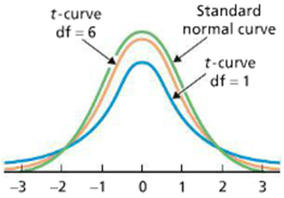
Definition: Probability density curve of a $T$-distribution

$clipboard_e82953a89eb5d550e2d20a01bb103641a.png$

The probability density curve of a $T$-distribution looks a lot like the standard normal probability density curve, and it has the following properties:

Property 1: The total area equals 1.

Property 2: Extends indefinitely in both directions, approaching, but never touching, the horizontal axis as it does so.

Property 3: Symmetric about 0.

Property 4: As the number of degrees of freedom becomes larger, t-curves look increasingly like the standard normal curve.

For example, let $T$ be a random variable that has $T$-distribution with $7$ degrees of freedom, then the probability density curve of $T$ takes a very specific shape determined by its parameter.

$clipboard_e34773eab90e144e86f38ba6e207a06d0.png$

Next, we want to be able to find $P(T<c)$ for all $c$ and find the $t_\alpha$’s for all $\alpha$. Let’s make sure we understand the questions well:

To find the probability $P(T<c)$ means to find the area under the $T$-curve to the left of $c$.
To find $t_\alpha$ means to find the value the area under the $T$-curve to the right of which is $\alpha$.

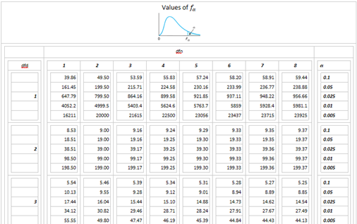
Luckily, there are many ways to use technology to answer these two questions. In reality, while it is not too hard to use technology to find the probabilities, very rarely one would have to do this task in the applications. However, while it is also not too hard to use technology to find $t_\alpha$’s, this task will be very common in the applications, so it is worth learning how to perform this task by hand. The most frequently used $t_\alpha$’s are summarized in the following table:

$clipboard_e71f060f1b02b613791c5d81b889f0c2b.png$

We only need to identify $\alpha$ and $df$, the degrees of freedom, then look for the value in the intersection.

Example $\PageIndex{2.1}$

For $T \sim T_{df=10}$, $t_{0.05}=1.895$.

For $T \sim T_{df=11}$, $t_{0.01}=2.718$.

How about $\alpha>0.5$? Turns out that while it is possible to create a table to summarize such $t_\alpha$’s there is no need for it. Since the $T$-distribution is symmetric about zero we can use the property of alpha-notation and conclude that

$t_\alpha=-t_{1-\alpha}$

Example $\PageIndex{2.2}$

For $T \sim T_{df=10}$, $t_{0.95}=-t_{0.05}=-1.895$.

For $T \sim T_{df=11}$, $t_{0.99}=-t_{0.01}=-2.718$.

Example $\PageIndex{2.3}$ with technology

The $z$-scores of the test results of a sample of students follow the $T$-distribution with $10$ degrees of freedom. Let $T$ be the $z$-score of a randomly selected student.

$T \sim T_{df=10}$

Find the probability that the z-score is:
1. less than $-0.75$: $P(T<-0.75)=0.235=23.5\%$
2. more than $2.5$: $P(T>2.5)=0.016=1.6\%$
3. between $-1$ and $1.33$: $P(-1<T<1.33)=0.723=72.3\%$
Compute the $95$-th percentile: $t_{95\%-th}=t_{0.05}=1.812$

Section 3: $X^2$-Distribution

Definition: Probability density curve of a $X^2$-distribution

$clipboard_eea3025a81dd6a77b39c8fa615550cab5.png$

The probability density curve of a $X^2$-distribution with $df$ degrees of freedom has the following properties:

Property 1: The total area equals 1.

Property 2: Starts at the origin and extends indefinitely to the right, approaching, but never touching, the horizontal axis.

Property 3: Right-skewed.

Property 4: As the number of degrees of freedom becomes larger, $X^2$-curves look increasingly like normal curves.

For example, let $X^2$ be a random variable that has $X^2$-distribution with $7$ degrees of freedom, then the probability density curve of $X^2$ takes a very specific shape determined by its parameter.

$clipboard_ed14599eaf30e8dd21ea7bcc5d19cf577.png$

Next, we want to be able to find $P(X^2<c)$ for all $c$ and find the $\chi_\alpha^2$’s for all $\alpha$. Let’s make sure we understand the questions well:

To find the probability $P(X^2<c)$ means to find the area under the $X^2$-curve to the left of $c$.
To find $\chi_\alpha^2$ means to find the value the area under the $X^2$-curve to the right of which is $\alpha$.

Luckily, there are many ways to use technology to answer these two questions. In reality, while it is not too hard to use technology to find the probabilities, very rarely one would have to do this task in the applications. However, while it is also not too hard to use technology to find $\chi_\alpha^2$, this task will be very common in the applications, so it is worth learning how to perform this task by hand. The most frequently used $\chi_\alpha^2$’s are summarized in the following table:

$clipboard_e9f055cda76dd53f4fdc1ee57a5ca0651.png$

We only need to identify $\alpha$ and $df$, the degrees of freedom, then look for the value in the intersection.

Example $\PageIndex{3.1}$

For $X^2 \sim X_{df=7}^2$, $\chi_{0.05}^2=14.067$.

For $X^2 \sim X_{df=12}^2$, $\chi_{0.01}^2=26.217$.

How about $\alpha>0.5$? Since $X^2$ is not symmetric about zero it is absolutely necessary to have a table to summarize such $\chi_\alpha^2$’s.

Example $\PageIndex{3.2}$

For $X^2 \sim X_{df=10}^2$, $\chi_{0.99}^2=2.558$.

Example $\PageIndex{3.3}$ with technology

A randomly selected car salesman’s annual salary (in thousands) can be estimated by a random variable that follows $X^2$-distribution with $df=40$. Let $X$ be the salary of a randomly selected car salesman.

$X \sim X_{df=40}^2$

Find the probability that the commission is:
1. less than $35K: $P(X<35)=0.305=30.5\%$
2. more than $50K: $P(X>50)=0.134=13.3\%$
3. between $40K and $60K: $P(40<X<60)=0.448=44.8\%$
Compute the 90-th percentile:$x_{90\%-th}=x_{0.1}=51.8$

Section 4: F-Distribution

Definition: Probability density curve of an $F$-distribution with parameters $(dfn,dfd)$

$clipboard_e2053753451d35a83e7b906ab984db246.png$

The probability density curve of an $F$-distribution with parameters $(dfn, dfd)$ has the following properties:

Property 1: The total area equals $1$.

Property 2: Starts at the origin and extends indefinitely to the right, approaching, but never touching, the horizontal axis.

Property 3: Right-skewed.

Property 4: The Reciprocal Property of $F$-Curves:

$f_\alpha=\frac{1}{f_{1-\alpha}^*}$ where $f^*$ has $df=(dfd, dfn)$

For example, let $F$ be a random variable that has $F$-distribution with $(6,2)$ degrees of freedom, then the probability density curve of $F$ takes a very specific shape determined by its parameter.

$clipboard_ea784d92a32a3af4f17993c1b0ef3d85c.png$

Next, we want to be able to find $P(F<c)$ for all $c$ and find the $f_\alpha$’s for all $\alpha$. Let’s make sure we understand the questions well:

To find the probability $P(F<c)$ means to find the area under the $F$-curve to the left of $c$.
To find $f_\alpha$ means to find the value the area under the $F$-curve to the right of which is $\alpha$.

Luckily, there are many ways to use technology to answer these two questions. In reality, while it is not too hard to use technology to find the probabilities, very rarely one would have to do this task in the applications. However, while it is also not too hard to use technology to find $f_\alpha$, this task will be very common in the applications, so it is worth learning how to perform this task by hand. The most frequently used $f_\alpha$’s are summarized in the following table:

$clipboard_e1e5c870bb23b62cca0c647a223e3bb9c.png$

We only need to identify $dfn$, $dfd$, and $\alpha$, then look for the value in the intersection.

Example $\PageIndex{4.1}$

For $F \sim F_{(6, 2)}$, $f_{0.05}=19.330$.

For $F \sim F_{(4, 3)}$, $f_{0.01}=28.71$

How about $\alpha>0.5$? Since $F$ is not symmetric about zero we can’t use the property of symmetric distributions, however we can use the reciprocal property of $F$-curves.

Example $\PageIndex{4.2}$

For $F \sim F_{(2, 3)}$, $f_{0.99}=\frac{1}{f_{0.01}^*}=frac{1}{99.17}=0.010$

Example $\PageIndex{4.3}$ with technology

A randomly selected realtor’s monthly commission (in thousands) can be estimated by a random variable that follows $F$-distribution with parameters $(15,3)$. Let $F$ be the commission of a randomly selected realtor.

$F \sim F_{(15, 3)}$

Find the probability that the commission is:
1. less than $1500: $P(F<1.5)=0.585=58.5\%$
2. more than $8000: $P(F>8)=0.056=5.6\%$
3. between $3000 and $7000: $P(3<F<7)=0.131=13.1\%$
Compute the median:$f_{50\%-th}=f_{0.5}=1.21$

Search

Text Color

Text Size

Margin Size

Font Type

Definition: Probability density curve of a \(T\)-distribution

Example \(\PageIndex{2.1}\)

Example \(\PageIndex{2.2}\)

Example \(\PageIndex{2.3}\) with technology

Definition: Probability density curve of a \(X^2\)-distribution

Example \(\PageIndex{3.1}\)

Example \(\PageIndex{3.2}\)

Example \(\PageIndex{3.3}\) with technology

Definition: Probability density curve of an \(F\)-distribution with parameters \((dfn,dfd)\)

Example \(\PageIndex{4.1}\)

Example \(\PageIndex{4.2}\)

Example \(\PageIndex{4.3}\) with technology