8.3: Normality Plots

Last updated
Save as PDF

Page ID: 105847

$ \newcommand{\vecs}[1]{\overset { \scriptstyle \rightharpoonup} {\mathbf{#1}} } $

$ \newcommand{\vecd}[1]{\overset{-\!-\!\rightharpoonup}{\vphantom{a}\smash {#1}}} $

$ \newcommand{\id}{\mathrm{id}}$ $ \newcommand{\Span}{\mathrm{span}}$

( \newcommand{\kernel}{\mathrm{null}\,}\) $ \newcommand{\range}{\mathrm{range}\,}$

$ \newcommand{\RealPart}{\mathrm{Re}}$ $ \newcommand{\ImaginaryPart}{\mathrm{Im}}$

$ \newcommand{\Argument}{\mathrm{Arg}}$ $ \newcommand{\norm}[1]{\| #1 \|}$

$ \newcommand{\inner}[2]{\langle #1, #2 \rangle}$

$ \newcommand{\Span}{\mathrm{span}}$

$ \newcommand{\id}{\mathrm{id}}$

$ \newcommand{\Span}{\mathrm{span}}$

$ \newcommand{\kernel}{\mathrm{null}\,}$

$ \newcommand{\range}{\mathrm{range}\,}$

$ \newcommand{\RealPart}{\mathrm{Re}}$

$ \newcommand{\ImaginaryPart}{\mathrm{Im}}$

$ \newcommand{\Argument}{\mathrm{Arg}}$

$ \newcommand{\norm}[1]{\| #1 \|}$

$ \newcommand{\inner}[2]{\langle #1, #2 \rangle}$

$ \newcommand{\Span}{\mathrm{span}}$ $ \newcommand{\AA}{\unicode[.8,0]{x212B}}$

$ \newcommand{\vectorA}[1]{\vec{#1}} % arrow$

$ \newcommand{\vectorAt}[1]{\vec{\text{#1}}} % arrow$

$ \newcommand{\vectorB}[1]{\overset { \scriptstyle \rightharpoonup} {\mathbf{#1}} } $

$ \newcommand{\vectorC}[1]{\textbf{#1}} $

$ \newcommand{\vectorD}[1]{\overrightarrow{#1}} $

$ \newcommand{\vectorDt}[1]{\overrightarrow{\text{#1}}} $

$ \newcommand{\vectE}[1]{\overset{-\!-\!\rightharpoonup}{\vphantom{a}\smash{\mathbf {#1}}}} $

$ \newcommand{\vecs}[1]{\overset { \scriptstyle \rightharpoonup} {\mathbf{#1}} } $

$ \newcommand{\vecd}[1]{\overset{-\!-\!\rightharpoonup}{\vphantom{a}\smash {#1}}} $

$\newcommand{\avec}{\mathbf a}$ $\newcommand{\bvec}{\mathbf b}$ $\newcommand{\cvec}{\mathbf c}$ $\newcommand{\dvec}{\mathbf d}$ $\newcommand{\dtil}{\widetilde{\mathbf d}}$ $\newcommand{\evec}{\mathbf e}$ $\newcommand{\fvec}{\mathbf f}$ $\newcommand{\nvec}{\mathbf n}$ $\newcommand{\pvec}{\mathbf p}$ $\newcommand{\qvec}{\mathbf q}$ $\newcommand{\svec}{\mathbf s}$ $\newcommand{\tvec}{\mathbf t}$ $\newcommand{\uvec}{\mathbf u}$ $\newcommand{\vvec}{\mathbf v}$ $\newcommand{\wvec}{\mathbf w}$ $\newcommand{\xvec}{\mathbf x}$ $\newcommand{\yvec}{\mathbf y}$ $\newcommand{\zvec}{\mathbf z}$ $\newcommand{\rvec}{\mathbf r}$ $\newcommand{\mvec}{\mathbf m}$ $\newcommand{\zerovec}{\mathbf 0}$ $\newcommand{\onevec}{\mathbf 1}$ $\newcommand{\real}{\mathbb R}$ $\newcommand{\twovec}[2]{\left[\begin{array}{r}#1 \\ #2 \end{array}\right]}$ $\newcommand{\ctwovec}[2]{\left[\begin{array}{c}#1 \\ #2 \end{array}\right]}$ $\newcommand{\threevec}[3]{\left[\begin{array}{r}#1 \\ #2 \\ #3 \end{array}\right]}$ $\newcommand{\cthreevec}[3]{\left[\begin{array}{c}#1 \\ #2 \\ #3 \end{array}\right]}$ $\newcommand{\fourvec}[4]{\left[\begin{array}{r}#1 \\ #2 \\ #3 \\ #4 \end{array}\right]}$ $\newcommand{\cfourvec}[4]{\left[\begin{array}{c}#1 \\ #2 \\ #3 \\ #4 \end{array}\right]}$ $\newcommand{\fivevec}[5]{\left[\begin{array}{r}#1 \\ #2 \\ #3 \\ #4 \\ #5 \\ \end{array}\right]}$ $\newcommand{\cfivevec}[5]{\left[\begin{array}{c}#1 \\ #2 \\ #3 \\ #4 \\ #5 \\ \end{array}\right]}$ $\newcommand{\mattwo}[4]{\left[\begin{array}{rr}#1 \amp #2 \\ #3 \amp #4 \\ \end{array}\right]}$ $\newcommand{\laspan}[1]{\text{Span}\{#1\}}$ $\newcommand{\bcal}{\cal B}$ $\newcommand{\ccal}{\cal C}$ $\newcommand{\scal}{\cal S}$ $\newcommand{\wcal}{\cal W}$ $\newcommand{\ecal}{\cal E}$ $\newcommand{\coords}[2]{\left\{#1\right\}_{#2}}$ $\newcommand{\gray}[1]{\color{gray}{#1}}$ $\newcommand{\lgray}[1]{\color{lightgray}{#1}}$ $\newcommand{\rank}{\operatorname{rank}}$ $\newcommand{\row}{\text{Row}}$ $\newcommand{\col}{\text{Col}}$ $\renewcommand{\row}{\text{Row}}$ $\newcommand{\nul}{\text{Nul}}$ $\newcommand{\var}{\text{Var}}$ $\newcommand{\corr}{\text{corr}}$ $\newcommand{\len}[1]{\left|#1\right|}$ $\newcommand{\bbar}{\overline{\bvec}}$ $\newcommand{\bhat}{\widehat{\bvec}}$ $\newcommand{\bperp}{\bvec^\perp}$ $\newcommand{\xhat}{\widehat{\xvec}}$ $\newcommand{\vhat}{\widehat{\vvec}}$ $\newcommand{\uhat}{\widehat{\uvec}}$ $\newcommand{\what}{\widehat{\wvec}}$ $\newcommand{\Sighat}{\widehat{\Sigma}}$ $\newcommand{\lt}{<}$ $\newcommand{\gt}{>}$ $\newcommand{\amp}{&}$ $\definecolor{fillinmathshade}{gray}{0.9}$

In a lot of problems in the future, it will be necessary to know whether the sample came from a normal population or not. Next, we will discuss how does one know whether the population is normal or not based on a sample.

We intuitively expect that the shape of the distribution of a sample is approximately the same as the shape of the population distribution. So if one can obtain a large representative sample (or the census) then the shape of its histogram will resemble the shape of the population's distribution. Therefore, if the distribution looks normal then it is an indicator that the sample came from a normal population. But what do we do when only a small sample can be obtained? In such a case, we will use a graph called a normality plot.

Turns out that normal populations are so common and well-studied that we almost know what to expect from a sample of any small size. The expectations are formulated in the following table:

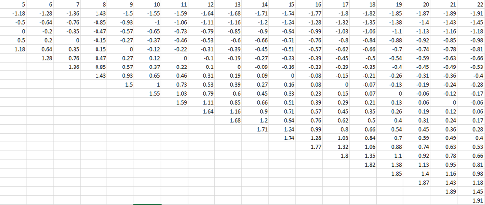
$clipboard_e45cd25f6d4e594d75e1e7eac9837604b.png$

This table provides the expected $z$-scores from a sample of each size from $5$ to $22$ in ascending order. So if we have the sample of size $5$, then we expect that one of the observations will be $1.18$ standard deviations below the mean, one of the observations will be $0.5$ standard deviations below the mean, one of the observations will be equal the mean, one of the observations will be $0.5$ standard deviations above the mean, one of the observations will be $1.18$ standard deviations above the mean.

Definition: Normality plot

To construct a normality plot:

Sort the sample of size $n$ in increasing order.
In the table of expected $z$-scores find the column corresponding to the sample size $n$.
List the expected $z$-scores from the table side-by-side with the observations in the sample.
Construct the scatterplot with expected $z$-scores as the input and the data as the output.

If the plot has a roughly linear pattern, you can assume that the sample came from a normally distributed population. If the plot is not roughly linear, you cannot assume that the sample is from a normal population. These guidelines should be interpreted loosely for smaller samples but usually strictly for larger samples.

Example $\PageIndex{1}$

A sample of five UBER drivers were asked how many hours they worked last week, and the following answers were obtained:

15, 12, 7, 3, 20

Use the normality plot to determine whether the population of weekly driving time is normal for UBER drivers.

Solution

$clipboard_e5ec36e2c26aba75aaa75d0e8fe193c7b.png$

Based on the shape of the normality plot we conclude that the sample came from a normal population.

Example $\PageIndex{2}$

A simple random sample of $12$ returns from last year revealed the adjusted gross incomes, in thousands of dollars, shown in the table below.

9.7	93.1	33.0	21.2
81.4	51.1	43.5	10.6
12.8	7.8	18.1	12.7

Construct a normal probability plot for these data and use the plot to assess the normality of adjusted gross incomes.

Solution

$clipboard_e41888dec7e2f62eb21c0de50d3be1cc5.png$

Based on the shape of the normality plot we conclude that the sample came from a not normal population.

When technology is not available to assess the normality just look at any visual representation of the sample data (dotplot, boxplot, stem-and-leaf, histogram etc.) and check the shape of the distribution for a symmetry, modality, and the outliers.

Search

Text Color

Text Size

Margin Size

Font Type

Solution

Solution

Definition: Normality plot

Example \(\PageIndex{1}\)

Solution

Example \(\PageIndex{2}\)

Solution