5.3: Line Integrals

Learning Objectives

• Calculate a scalar line integral along a curve.
• Calculate a vector line integral along an oriented curve in space.
• Use a line integral to compute the work done in moving an object along a curve in a vector field.
• Describe the flux and circulation of a vector field.

We are familiar with single-variable integrals of the form $\displaystyle \int_{a}^{b}f(x)\,dx$, where the domain of integration is an interval $[a,b]$. Such an interval can be thought of as a curve in the $xy$-plane, since the interval defines a line segment with endpoints $(a,0)$ and $(b,0)$—in other words, a line segment located on the $x$-axis. Suppose we want to integrate over any curve in the plane, not just over a line segment on the $x$-axis. Such a task requires a new kind of integral, called a line integral.

Line integrals have many applications to engineering and physics. They also allow us to make several useful generalizations of the Fundamental Theorem of Calculus. And, they are closely connected to the properties of vector fields, as we shall see.

Scalar Line Integrals

A line integral gives us the ability to integrate multivariable functions and vector fields over arbitrary curves in a plane or in space. There are two types of line integrals: scalar line integrals and vector line integrals. Scalar line integrals are integrals of a scalar function over a curve in a plane or in space. Vector line integrals are integrals of a vector field over a curve in a plane or in space. Let’s look at scalar line integrals first.

A scalar line integral is defined just as a single-variable integral is defined, except that for a scalar line integral, the integrand is a function of more than one variable and the domain of integration is a curve in a plane or in space, as opposed to a curve on the $x$-axis.

For a scalar line integral, we let $C$ be a smooth curve in a plane or in space and let $f$ be a function with a domain that includes $C$. We chop the curve into small pieces. For each piece, we choose point $P$ in that piece and evaluate $f$ at $P$. (We can do this because all the points in the curve are in the domain of $f$.) We multiply $f(P)$ by the arc length of the piece $\Delta s$, add the product $f(P)\Delta s$ over all the pieces, and then let the arc length of the pieces shrink to zero by taking a limit. The result is the scalar line integral of the function over the curve.

For a formal description of a scalar line integral, let $C$ be a smooth curve in space given by the parameterization $\vecs r(t)=⟨x(t),y(t),z(t)⟩$, $a≤t≤b$. Let $f(x,y,z)$ be a function with a domain that includes curve $C$. To define the line integral of the function $f$ over $C$, we begin as most definitions of an integral begin: we chop the curve into small pieces. Partition the parameter interval $[a,b]$ into $n$ subintervals $[t_{i−l},t_i]$ of equal width for $1≤i≤n$, where $t_0=a$ and $t_n=b$ (Figure $\PageIndex{1}$). Let $t_{i}^*$ be a value in the $i^{th}$ interval $[t_{i−l},t_i]$. Denote the endpoints of $\vecs r(t_0)$, $\vecs r(t_1)$,…, $\vecs r(t_n)$ by $P_0$,…, $P_n$. Points P_i divide curve $C$ into $n$ pieces $C_1$, $C_2$,…, $C_n$,with lengths $\Delta s_1$, $\Delta s_2$,…, $\Delta s_n$, respectively. Let $P_{i}^*$ denote the endpoint of $\vecs r(t_{i}^*)$ for $1≤i≤n$. Now, we evaluate the function $f$ at point $P_{i}^*$ for $1≤i≤n$. Note that $P_{i}^*$ is in piece $C_1$, and therefore $P_{i}^*$ is in the domain of $f$. Multiply $f(P_{i}^*)$ by the length $\Delta s_1$ of $C_1$, which gives the area of the “sheet” with base $C_1$, and height $f(P_{i}^{*})$. This is analogous to using rectangles to approximate area in a single-variable integral. Now, we form the sum $\displaystyle \sum_{i=1}^{n} f(P_{i}^{*})\,\Delta s_i$.

Figure $\PageIndex{1}$: Curve $C$ has been divided into n pieces, and a point inside each piece has been chosen.

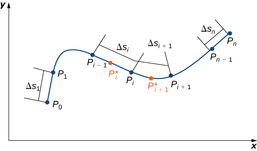
Note the similarity of this sum versus a Riemann sum; in fact, this definition is a generalization of a Riemann sum to arbitrary curves in space. Just as with Riemann sums and integrals of form $\displaystyle \int_{a}^{b}g(x)\,dx$, we define an integral by letting the width of the pieces of the curve shrink to zero by taking a limit. The result is the scalar line integral of $f$ along $C$.

You may have noticed a difference between this definition of a scalar line integral and a single-variable integral. In this definition, the arc lengths $\Delta s_1$, $\Delta s_2$,…, $\Delta s_n$ aren’t necessarily the same; in the definition of a single-variable integral, the curve in the $x$-axis is partitioned into pieces of equal length. This difference does not have any effect in the limit. As we shrink the arc lengths to zero, their values become close enough that any small difference becomes irrelevant.

DEFINITION: Scalar Line Integral

Let $f$ be a function with a domain that includes the smooth curve $C$ that is parameterized by $\vecs r(t)=⟨x(t),y(t),z(t)⟩$, $a≤t≤b$. The scalar line integral of $f$ along $C$ is

$$\int_C f(x,y,z) \,ds=\lim_{n\to\infty}\sum_{i=1}^{n}f(P_{i}^{*})\,\Delta s_i \label{eq12a}$$

if this limit exists ($t_i ^{*}$ and $\Delta s_i$ are defined as in the previous paragraphs). If $C$ is a planar curve, then $C$ can be represented by the parametric equations $x=x(t)$, $y=y(t)$, and $a≤t≤b$. If $C$ is smooth and $f(x,y)$ is a function of two variables, then the scalar line integral of $f$ along $C$ is defined similarly as

$$\int_C f(x,y) \,ds=\lim_{n\to\infty}\sum_{i=1}^{n} f(P_{i}^{*})\,\Delta s_i, \label{eq13}$$

if this limit exists.

If $f$ is a continuous function on a smooth curve $C$, then $\displaystyle \int_C f \,ds$ always exists. Since $\displaystyle \int_C f \,ds$ is defined as a limit of Riemann sums, the continuity of $f$ is enough to guarantee the existence of the limit, just as the integral $\displaystyle \int_{a}^{b}g(x)\,dx$ exists if $g$ is continuous over $[a,b]$.

Before looking at how to compute a line integral, we need to examine the geometry captured by these integrals. Suppose that $f(x,y)≥0$ for all points $(x,y)$ on a smooth planar curve $C$. Imagine taking curve $C$ and projecting it “up” to the surface defined by $f(x,y)$, thereby creating a new curve $C′$ that lies in the graph of $f(x,y)$ (Figure $\PageIndex{2}$). Now we drop a “sheet” from $C′$ down to the $xy$-plane. The area of this sheet is $\displaystyle \int_C f(x,y)ds$. If $f(x,y)≤0$ for some points in $C$, then the value of $\displaystyle \int_C f(x,y)\,ds$ is the area above the $xy$-plane less the area below the $xy$-plane. (Note the similarity with integrals of the form $\displaystyle \int_{a}^{b}g(x)\,dx$.)

Figure $\PageIndex{2}$: The area of the blue sheet is $\displaystyle \int_C f(x,y)\,ds$.

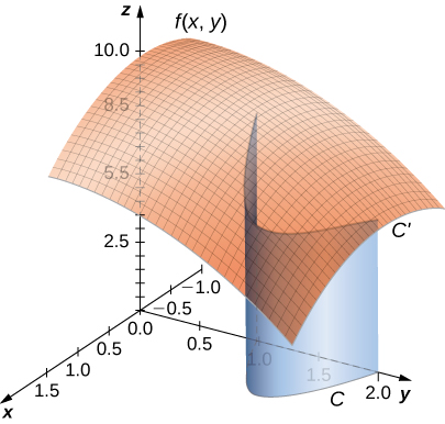
From this geometry, we can see that line integral $\displaystyle \int_C f(x,y)\,ds$ does not depend on the parameterization $\vecs r(t)$ of $C$. As long as the curve is traversed exactly once by the parameterization, the area of the sheet formed by the function and the curve is the same. This same kind of geometric argument can be extended to show that the line integral of a three-variable function over a curve in space does not depend on the parameterization of the curve.

Example $\PageIndex{1}$: ​​​​​​Finding the Value of a Line Integral

Find the value of integral $\displaystyle \int_C 2\,ds$, where $C$ is the upper half of the unit circle.

Solution

The integrand is $f(x,y)=2$. Figure $\PageIndex{3}$ shows the graph of $f(x,y)=2$, curve C, and the sheet formed by them. Notice that this sheet has the same area as a rectangle with width $\pi$ and length $2$. Therefore, $\displaystyle \int_C 2 \,ds=2\pi\,\text{units}^2$.

Figure $\PageIndex{3}$: The sheet that is formed by the upper half of the unit circle in a plane and the graph of $f(x,y)=2$.

To see that $\displaystyle \int_C 2 \,ds=2\pi$ using the definition of line integral, we let $\vecs r(t)$ be a parameterization of $C$. Then, $f(\vecs r(t_i))=2$ for any number $t_i$ in the domain of $\vecs r$. Therefore,

$$\begin{align*} \int_C f \,ds &=\lim_{n\to\infty}\sum_{i=1}^{n} f(\vecs r(t_{i}^{*}))\,\Delta s_i \\[4pt] &=\lim_{n\to\infty}\sum_{i=1}^{n}2\,\Delta s_i \\[4pt] &=2\lim_{n\to\infty}\sum_{i=1}^{n}\,\Delta s_i \\[4pt] &=2(\text{length}\space \text{of}\space C) \\[4pt] &=2\pi \,\text{units}^2. \end{align*}$$

Exercise $\PageIndex{1}$

Find the value of $\displaystyle \int_C(x+y)\,ds$, where $C$ is the curve parameterized by $x=t$, $y=t$, $0≤t≤1$.

Hint

Find the shape formed by $C$ and the graph of function $f(x,y)=x+y$.

Answer

$\sqrt{2}$

Note that in a scalar line integral, the integration is done with respect to arc length $s$, which can make a scalar line integral difficult to calculate. To make the calculations easier, we can translate $\displaystyle \int_C f\,ds$ to an integral with a variable of integration that is $t$.

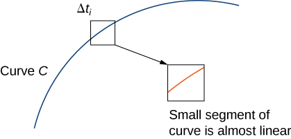
Let $\vecs r(t)=⟨x(t),y(t),z(t)⟩$ for $a≤t≤b$ be a parameterization of $C$. Since we are assuming that $C$ is smooth, $\vecs r′(t)=⟨x′(t),y′(t),z′(t)⟩$ is continuous for all $t$ in $[a,b]$. In particular, $x′(t)$, $y′(t)$, and $z′(t)$ exist for all $t$ in $[a,b]$. According to the arc length formula, we have

$$\text{length}(C_i)=\Delta s_i=\int_{t_{i−1}}^{t_i} ‖\vecs r′(t)‖\,dt. \nonumber$$

If width $\Delta t_i=t_i−t_{i−1}$ is small, then function $\displaystyle \int_{t_{i−1}}^{t_i} ‖\vecs r′(t)‖\,dt\,≈\,‖\vecs r′(t_i^*)‖\,\Delta t_i$, $‖\vecs r′(t)‖$ is almost constant over the interval $[t_{i−1},t_i]$.Therefore,

$$\int_{t_{i−1}}^{t_i} ‖\vecs r′(t)‖\,dt\,≈\,‖\vecs r′(t_{i}^{*})‖\,\Delta t_i, \label{approxLineIntEq1}$$

and we have

$$\sum_{i=1}^{n} f(\vecs r(t_i^*))\,\Delta s_i\approx\sum_{i=1}^{n} f(\vecs r(t_{i}^{*})) ‖\vecs r′(t_{i}^{*})‖\,\Delta t_i. \nonumber$$

See Figure $\PageIndex{4}$.

Figure $\PageIndex{4}$: If we zoom in on the curve enough by making $\Delta t_i$ very small, then the corresponding piece of the curve is approximately linear.

Note that

$$\lim_{n\to\infty}\sum_{i=1}^{n} f(\vecs r(t_i^*))‖\vecs r′(t_{i}^{*})‖\,\Delta t_i=\int_a^b f(\vecs r(t))‖\vecs r′(t)‖\,dt. \nonumber$$

In other words, as the widths of intervals $[t_{i−1},t_i]$ shrink to zero, the sum $\displaystyle \sum_{i=1}^{n} f(\vecs r(t_i^{*}))‖\vecs r′(t_{i}^{*})‖\,\Delta t_i$ converges to the integral $\displaystyle \int_{a}^{b}f(\vecs r(t))‖\vecs r′(t)‖\,dt$. Therefore, we have the following theorem.

Theorem: Evaluating a Scalar Line Integral

Let $f$ be a continuous function with a domain that includes the smooth curve $C$ with parameterization $\vecs r(t)$, $a≤t≤b$. Then

$$\int_C f \,ds=\int_{a}^{b} f(\vecs r(t))‖\vecs r′(t)‖\,dt.\label{scalerLineInt1}$$

Although we have labeled Equation $\ref{approxLineIntEq1}$ as an equation, it is more accurately considered an approximation because we can show that the left-hand side of Equation $\ref{approxLineIntEq1}$ approaches the right-hand side as $n\to\infty$. In other words, letting the widths of the pieces shrink to zero makes the right-hand sum arbitrarily close to the left-hand sum. Since

$$‖\vecs r′(t)‖=\sqrt{{(x′(t))}^2+{(y′(t))}^2+{(z′(t))}^2}, \nonumber$$

we obtain the following theorem, which we use to compute scalar line integrals.

Theorem: Scalar Line Integral Calculation

Let $f$ be a continuous function with a domain that includes the smooth curve $C$ with parameterization $\vecs r(t)=⟨x(t),y(t),z(t)⟩$, $a≤t≤b$. Then

$$\int_C f(x,y,z) \,ds=\int_{a}^{b} f(\vecs r(t))\sqrt{({x′(t))}^2+{(y′(t))}^2+{(z′(t))}^2} \,dt. \nonumber$$

Similarly,

$$\int_C f(x,y) \,ds=\int_{a}^{b}f(\vecs r(t))\sqrt{{(x′(t))}^2+{(y′(t))}^2} \,dt \nonumber$$

if $C$ is a planar curve and $f$ is a function of two variables.

Note that a consequence of this theorem is the equation $ds=‖\vecs r′(t)‖ \,dt$. In other words, the change in arc length can be viewed as a change in the $t$-domain, scaled by the magnitude of vector $\vecs r′(t)$.

Example $\PageIndex{2}$: Evaluating a Line Integral

Find the value of integral $\displaystyle \int_C(x^2+y^2+z) \,ds$, where $C$ is part of the helix parameterized by $\vecs r(t)=⟨\cos t,\sin t,t⟩$, $0≤t≤2\pi$.

Solution

To compute a scalar line integral, we start by converting the variable of integration from arc length $s$ to $t$. Then, we can use Equation $\ref{eq12a}$ to compute the integral with respect to $t$. Note that

$$f(\vecs r(t))={\cos}^2 t+{\sin}^2 t+t=1+t \nonumber$$

and

$$\sqrt{{(x′(t))}^2+{(y′(t))}^2+{(z′(t))}^2} =\sqrt{{(−\sin(t))}^2+{\cos}^2(t)+1} =\sqrt{2}.\nonumber$$

Therefore,

$$\int_C(x^2+y^2+z) \,ds=\int_{0}^{2\pi} (1+t)\sqrt{2} \,dt. \nonumber$$

Notice that Equation $\ref{eq12a}$ translated the original difficult line integral into a manageable single-variable integral. Since

$$\begin{align*} \int_{0}^{2\pi} (1+t)\sqrt{2}\, dt &={\left[\sqrt{2}t+\dfrac{\sqrt{2}t^2}{2}\right]}_{0}^{2\pi} \\[4pt] &=2\sqrt{2}\pi+2\sqrt{2}{\pi}^2, \end{align*}$$

we have

$$\int_C(x^2+y^2+z) \,ds=2\sqrt{2}\pi+2\sqrt{2}{\pi}^2. \nonumber$$

Exercise $\PageIndex{2}$

Evaluate $\displaystyle \int_C(x^2+y^2+z)ds$, where C is the curve with parameterization $\vecs r(t)=⟨\sin(3t),\cos(3t)⟩$, $0≤t≤\dfrac{\pi}{4}$.

Hint

Use the two-variable version of scalar line integral definition (Equation $\ref{eq13}$).

Answer

$$\dfrac{1}{3}+\dfrac{\sqrt{2}}{6}+\dfrac{3\pi}{4} \nonumber$$

Example $\PageIndex{3}$: Independence of Parameterization

Find the value of integral $\displaystyle \int_C(x^2+y^2+z) \,ds$, where $C$ is part of the helix parameterized by $\vecs r(t)=⟨\cos(2t),\sin(2t),2t⟩$, $0≤t≤π$. Notice that this function and curve are the same as in the previous example; the only difference is that the curve has been reparameterized so that time runs twice as fast.

Solution

As with the previous example, we use Equation $\ref{eq12a}$ to compute the integral with respect to $t$. Note that $f(\vecs r(t))={\cos}^2(2t)+{\sin}^2(2t)+2t=2t+1$ and

$$\begin{align*} \sqrt{{(x′(t))}^2+{(y′(t))}^2+{(z′(t))}^2} &=\sqrt{(−\sin t+\cos t+4)} \\[4pt] &=22 \end{align*}$$

so we have

$$\begin{align*} \int_C(x^2+y^2+z)ds &=2\sqrt{2}\int_{0}^{\pi}(1+2t)dt\\[4pt] &=2\sqrt{2}\Big[t+t^2\Big]_0^{\pi} \\[4pt] &=2\sqrt{2}(\pi+{\pi}^2). \end{align*}$$

Notice that this agrees with the answer in the previous example. Changing the parameterization did not change the value of the line integral. Scalar line integrals are independent of parameterization, as long as the curve is traversed exactly once by the parameterization.

Exercise $\PageIndex{3}$

Evaluate line integral $\displaystyle \int_C(x^2+yz) \,ds$, where $C$ is the line with parameterization $\vecs r(t)=⟨2t,5t,−t⟩$, $0≤t≤10$. Reparameterize C with parameterization $s(t)=⟨4t,10t,−2t⟩$, $0≤t≤5$, recalculate line integral $\displaystyle \int_C(x^2+yz) \,ds$, and notice that the change of parameterization had no effect on the value of the integral.

Hint

Use Equation $\ref{eq12a}$.

Answer

Both line integrals equal $−\dfrac{1000\sqrt{30}}{3}$.

Now that we can evaluate line integrals, we can use them to calculate arc length. If $f(x,y,z)=1$, then

$$\begin{align*} \int_C f(x,y,z) \,ds &=\lim_{n\to\infty} \sum_{i=1}^{n} f(t_{i}^{*}) \,\Delta s_i \\[4pt] &=\lim_{n\to\infty} \sum_{i=1}^{n} \,\Delta s_i \\[4pt] &=\lim_{n\to\infty} \text{length} (C)\\[4pt] &=\text{length} (C). \end{align*}$$

Therefore, $\displaystyle \int_C 1 \,ds$ is the arc length of $C$.

Example $\PageIndex{4}$: Calculating Arc Length

A wire has a shape that can be modeled with the parameterization $\vecs r(t)=⟨\cos t,\sin t,\frac{2}{3} t^{3/2}⟩$, $0≤t≤4\pi$. Find the length of the wire.

Solution

The length of the wire is given by $\displaystyle \int_C 1 \,ds$, where $C$ is the curve with parameterization $\vecs r$. Therefore,

$$\begin{align*} \text{The length of the wire} &=\int_C 1 \,ds \\[4pt] &=\int_{0}^{4\pi} ||\vecs r′(t)||\,dt \\[4pt] &=\int_{0}^{4\pi} \sqrt{(−\sin t)^2+\cos^2 t+t}dt \\[4pt] &=\int_{0}^{4\pi} \sqrt{1+t} dt \\[4pt] &=\left.\dfrac{2{(1+t)}^{\frac{3}{2}}}{3} \right|_{0}^{4\pi} \\[4pt] &=\frac{2}{3}\left((1+4\pi)^{3/2}−1\right). \end{align*}$$

Exercise $\PageIndex{4}$

Find the length of a wire with parameterization $\vecs r(t)=⟨3t+1,4−2t,5+2t⟩$, $0≤t≤4$.

Hint

Find the line integral of one over the corresponding curve.

Answer

$4\sqrt{17}$