5.3.1: Line Integrals - Part 2

In this part of the section, we are going to develop a second type of line integral called a vector line integral.  Although it's result is also a scalar, it is defined a little differently than the scalar line integral defined earlier in this section.  The previous definition is repeated below for easy reference.

DEFINITION: Scalar Line Integral

Let \(f\) be a function with a domain that includes the smooth curve \(C\) that is parameterized by \(\vecs r(t)=⟨x(t),y(t),z(t)⟩\), \(a≤t≤b\). The scalar line integral of \(f\) along \(C\) is

\[\int_C f(x,y,z) \,ds=\lim_{n\to\infty}\sum_{i=1}^{n}f(P_{i}^{*})\,\Delta s_i \label{eq12a}\]

if this limit exists \(t_{i}^{*}\) and \(\Delta s_i\) are defined as in the previous paragraphs). If \(C\) is a planar curve, then \(C\) can be represented by the parametric equations \(x=x(t)\), \(y=y(t)\), and \(a≤t≤b\). If \(C\) is smooth and \(f(x,y)\) is a function of two variables, then the scalar line integral of \(f\) along \(C\) is defined similarly as

\[\int_C f(x,y) \,ds=\lim_{n\to\infty}\sum_{i=1}^{n} f(P_{i}^{*})\,\Delta s_i, \label{eq13}\]

if this limit exists.

 

Vector Line Integrals

The second type of line integrals are vector line integrals, in which we integrate along a curve through a vector field. For example, let

\[\vecs F(x,y,z)=P(x,y,z)\,\hat{\mathbf i}+Q(x,y,z)\,\hat{\mathbf j}+R(x,y,z)\,\hat{\mathbf k} \nonumber \]

be a continuous vector field in \(ℝ^3\) that represents a force on a particle, and let \(C\) be a smooth curve in \(ℝ^3\) contained in the domain of \(\vecs F\). How would we compute the work done by \(\vecs F\) in moving a particle along \(C\)?

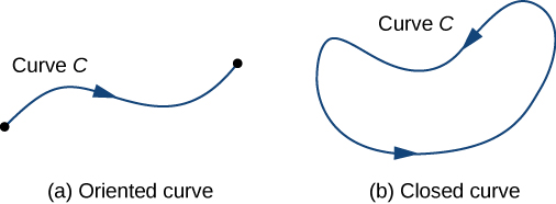
To answer this question, first note that a particle could travel in two directions along a curve: a forward direction and a backward direction. The work done by the vector field depends on the direction in which the particle is moving. Therefore, we must specify a direction along curve \(C\); such a specified direction is called an orientation of a curve. The specified direction is the positive direction along \(C\); the opposite direction is the negative direction along \(C\). When \(C\) has been given an orientation, \(C\) is called an oriented curve (Figure \(\PageIndex{5}\)). The work done on the particle depends on the direction along the curve in which the particle is moving.

A closed curve is one for which there exists a parameterization \(\vecs r(t)\), \(a≤t≤b\), such that \(\vecs r(a)=\vecs r(b)\), and the curve is traversed exactly once. In other words, the parameterization is one-to-one on the domain \((a,b)\).

Figure \(\PageIndex{5}\): (a) An oriented curve between two points. (b) A closed oriented curve.

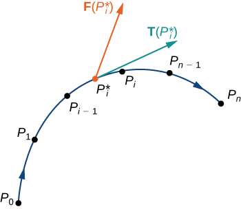
Let \(\vecs r(t)\) be a parameterization of \(C\) for \(a≤t≤b\) such that the curve is traversed exactly once by the particle and the particle moves in the positive direction along \(C\). Divide the parameter interval \([a,b]\) into n subintervals \([t_{i−1},t_i]\), \(0≤i≤n\), of equal width. Denote the endpoints of \(r(t_0)\), \(r(t_1)\),…, \(r(t_n)\) by \(P_0\),…,\(P_n\). Points \(P_i\) divide \(C\) into n pieces. Denote the length of the piece from \(P_{i−1}\) to \(P_i\) by \(\Delta s_i\). For each \(i\), choose a value \(t_i^*\) in the subinterval \([t_{i−1},t_i]\). Then, the endpoint of \(\vecs r(t_i^*)\) is a point in the piece of \(C\) between \(P_{i−1}\) and \(P_i\) (Figure \(\PageIndex{6}\)). If \(\Delta s_i\) is small, then as the particle moves from \(P_{i−1}\) to \(P_i\) along \(C\), it moves approximately in the direction of \(\vecs T(P_i)\), the unit tangent vector at the endpoint of \(\vecs r(t_i^*)\). Let \(P_i^*\) denote the endpoint of \(\vecs r(t_i^*)\). Then, the work done by the force vector field in moving the particle from \(P_{i−1}\) to \(P_i\) is \(\vecs F(P_i^*)·(\Delta s_i \vecs T(P_i^*))\), so the total work done along \(C\) is

\[\sum_{i=1}^n \vecs F(P_i^*)·(\Delta s_i \vecs T(P_i^*))=\sum_{i=1}^n \vecs F(P_i^*)·\vecs T(P_i^*)\,\Delta s_i. \nonumber \]

Figure \(\PageIndex{6}\): Curve \(C\) is divided into n pieces, and a point inside each piece is chosen. The dot product of any tangent vector in the ith piece with the corresponding vector \(\vecs{F}\) is approximated by \(\vecs{F}(P_i^*) \cdot \vecs{T}(P_i^*)\).

Letting the arc length of the pieces of \(C\) get arbitrarily small by taking a limit as \(n\rightarrow \infty\) gives us the work done by the field in moving the particle along \(C\). Therefore, the work done by \(\vecs{F}\) in moving the particle in the positive direction along \(C\) is defined as

\[W=\int_C \vecs{F} \cdot \vecs{T}\,ds, \nonumber \]

which gives us the concept of a vector line integral.

DEFINITION: Line Integral of a Vector Field

The vector line integral of vector field \(\vecs{F}\) along oriented smooth curve \(C\) is

\[\int_C \vecs{F} \cdot \vecs{T}\, ds=\lim_{n\to\infty} \sum_{i=1}^{n} \vecs{F}(P_i^*) \cdot \vecs{T}(P_i^*)\Delta s_i \nonumber \]

if that limit exists.

With scalar line integrals, neither the orientation nor the parameterization of the curve matters. As long as the curve is traversed exactly once by the parameterization, the value of the line integral is unchanged. With vector line integrals, the orientation of the curve does matter. If we think of the line integral as computing work, then this makes sense: if you hike up a mountain, then the gravitational force of Earth does negative work on you. If you walk down the mountain by the exact same path, then Earth’s gravitational force does positive work on you. In other words, reversing the path changes the work value from negative to positive in this case. Note that if \(C\) is an oriented curve, then we let \(−C\) represent the same curve but with opposite orientation.

As with scalar line integrals, it is easier to compute a vector line integral if we express it in terms of the parameterization function \(\vecs{r}\) and the variable \(t\). To translate the integral \(\displaystyle \int_C \vecs{F} \cdot \vecs{T}ds\) in terms of \(t\), note that unit tangent vector \(\vecs{T}\) along \(C\) is given by \(\vecs{T}=\dfrac{\vecs{r}′(t)}{‖\vecs{r}′(t)‖}\) (assuming \(‖\vecs{r}′(t)‖≠0\)). Since \(ds=‖\vecs r′(t)‖\,dt\), as we saw when discussing scalar line integrals, we have

\[\vecs F·\vecs T\,ds=\vecs F(\vecs r(t))·\dfrac{\vecs r′(t)}{‖\vecs r′(t)‖}‖\vecs r′(t)‖dt=\vecs F(\vecs r(t))·\vecs r′(t)\,dt. \nonumber \]

Thus, we have the following formula for computing vector line integrals:

\[\int_C\vecs F·\vecs T\,ds=\int_a^b \vecs F(\vecs r(t))·\vecs r′(t)\,dt.\label{lineintformula} \]

Because of Equation \ref{lineintformula}, we often use the notation \(\displaystyle \int_C \vecs{F} \cdot d\vecs{r}\) for the line integral \(\displaystyle \int_C \vecs F·\vecs T\,ds\).

If \(\vecs r(t)=⟨x(t),y(t),z(t)⟩\), then \(\dfrac{d\vecs{r}}{dt}\) denotes vector \(⟨x′(t),y′(t),z′(t)⟩\), and \(d\vecs{r} = \vecs r'(t)\,dt\).

Example \(\PageIndex{5}\): Evaluating a Vector Line Integral

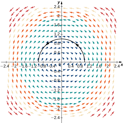
Find the value of integral \(\displaystyle \int_C \vecs{F} \cdot d\vecs{r}\), where \(C\) is the semicircle parameterized by \(\vecs{r}(t)=⟨\cos t,\sin t⟩\), \(0≤t≤\pi\) and \(\vecs F=⟨−y,x⟩\).

Solution

We can use Equation \ref{lineintformula} to convert the variable of integration from \(s\) to \(t\). We then have

\[\vecs F(\vecs r(t))=⟨−\sin t,\cos t⟩ \; \text{and} \; \vecs r′(t)=⟨−\sin t,\cos t⟩ . \nonumber \]

Therefore,

\[\begin{align*} \int_C \vecs{F} \cdot d\vecs{r} &=\int_0^{\pi}⟨−\sin t,\cos t⟩·⟨−\sin t,\cos t⟩ \,dt \\[4pt] &=\int_0^{\pi} {\sin}^2 t+{\cos}^2 t \,dt \\[4pt] &=\int_0^{\pi}1 \,dt=\pi.\end{align*}\]

See Figure \(\PageIndex{7}\).

Figure \(\PageIndex{7}\): This figure shows curve \(\vecs r(t)=⟨\cos t,\,\sin t⟩\), \(0≤t≤\pi\) in vector field \(\vecs F=⟨−y,\,x⟩\).

Example \(\PageIndex{6}\): Reversing Orientation

Find the value of integral \(\displaystyle \int_C \vecs{F} \cdot d\vecs{r}\), where \(C\) is the semicircle parameterized by \(\vecs r(t)=⟨\cos (t+π),\sin t⟩\), \(0≤t≤\pi\) and \(\vecs F=⟨−y,x⟩\).

Solution

Notice that this is the same problem as Example \(\PageIndex{5}\), except the orientation of the curve has been traversed. In this example, the parameterization starts at \(\vecs r(0)=⟨-1,0⟩\) and ends at \(\vecs r(\pi)=⟨1,0⟩\). By Equation \ref{lineintformula},

\[\begin{align*} \int_C \vecs{F} \cdot d\vecs{r} &=\int_0^{\pi} ⟨−\sin t,\cos (t+\pi)⟩·⟨−\sin (t+\pi), \cos t⟩dt\\[4pt] &=\int_0^{\pi}⟨−\sin t,−\cos t⟩·⟨\sin t,\cos t⟩dt\\[4pt] &=\int_{0}^{π}(−{\sin}^2 t−{\cos}^2 t)dt \\[4pt] &=\int_{0}^{\pi}−1dt\\[4pt] &=−\pi. \end{align*}\]

Notice that this is the negative of the answer in Example \(\PageIndex{5}\). It makes sense that this answer is negative because the orientation of the curve goes against the “flow” of the vector field.

Let \(C\) be an oriented curve and let \(-C\) denote the same curve but with the orientation reversed. Then, the previous two examples illustrate the following fact:

\[\int_{-C} \vecs{F} \cdot d\vecs{r}=−\int_C\vecs{F} \cdot d\vecs{r}. \nonumber \]

That is, reversing the orientation of a curve changes the sign of a line integral.

Exercise \(\PageIndex{6}\)

Let \(\vecs F=x\,\hat{\mathbf i}+y \,\hat{\mathbf j}\) be a vector field and let \(C\) be the curve with parameterization \(⟨t,t^2⟩\) for \(0≤t≤2\). Which is greater: \(\displaystyle \int_C\vecs F·\vecs T\,ds\) or \(\displaystyle \int_{−C} \vecs F·\vecs T\,ds\)?

Hint

Imagine moving along the path and computing the dot product \(\vecs F·\vecs T\) as you go.

Answer

\[\int_C \vecs F·\vecs T \,ds \nonumber \]

Another standard notation for integral \(\displaystyle \int_C \vecs{F} \cdot d\vecs{r}\) is \(\displaystyle \int_C P\,dx+Q\,dy+R \,dz\). In this notation, \(P,\, Q\), and \(R\) are functions, and we think of \(d\vecs{r}\) as vector \(⟨dx,dy,dz⟩\). To justify this convention, recall that \(d\vecs{r}=\vecs T\,ds=\vecs r′(t) \,dt=\left\langle\dfrac{dx}{dt},\dfrac{dy}{dt},\dfrac{dz}{dt}\right\rangle\,dt\). Therefore,

\[\vecs{F} \cdot d\vecs{r}=⟨P,Q,R⟩·⟨dx,dy,dz⟩=P\,dx+Q\,dy+R\,dz. \nonumber \]

If \(d\vecs{r}=⟨dx,dy,dz⟩\), then \(\dfrac{dr}{dt}=\left\langle\dfrac{dx}{dt},\dfrac{dy}{dt},\dfrac{dz}{dt}\right\rangle\), which implies that \(d\vecs{r}=\left\langle\dfrac{dx}{dt},\dfrac{dy}{dt},\dfrac{dz}{dt}\right\rangle\,dt\). Therefore

\[\begin{align} \int_C \vecs{F} \cdot d\vecs{r} &=\int_C P\,dx+Q\,dy+R\,dz \\[4pt] &=\int_a^b\left(P\big(\vecs r(t)\big)\dfrac{dx}{dt}+Q\big(\vecs r(t)\big)\dfrac{dy}{dt}+R\big(\vecs r(t)\big)\dfrac{dz}{dt}\right)\,dt. \label{eq14}\end{align} \]

Example \(\PageIndex{7}\): Finding the Value of an Integral of the Form \(\displaystyle \int_C P\,dx+Q\,dy+R\,dz\)

Find the value of integral \(\displaystyle \int_C z\,dx+x\,dy+y\,dz\), where \(C\) is the curve parameterized by \(\vecs r(t)=⟨t^2,\sqrt{t},t⟩\), \(1≤t≤4\).

Solution

As with our previous examples, to compute this line integral we should perform a change of variables to write everything in terms of \(t\). In this case, Equation \ref{eq14} allows us to make this change:

\[\begin{align*} \int_C z\,dx+x\,dy+y\,dz &=\int_1^4 \left(t(2t)+t^2\left(\frac{1}{2\sqrt{t}}\right)+\sqrt{t}\right)\,dt \\[4pt] &=\int_1^4\left(2t^2+\frac{t^{3/2}}{2}+\sqrt{t}\right)\,dt \\[4pt] &={\left[\dfrac{2t^3}{3}+\dfrac{t^{5/2}}{5}+\dfrac{2t^{3/2}}{3} \right]}_{t=1}^{t=4} \\[4pt] &=\dfrac{793}{15}.\end{align*}\]

Exercise \(\PageIndex{7}\)

Find the value of \(\displaystyle \int_C 4x\,dx+z\,dy+4y^2\,dz\), where \(C\) is the curve parameterized by \(\vecs r(t)=⟨4\cos(2t),2\sin(2t),3⟩\), \(0≤t≤\dfrac{\pi}{4}\).

Hint

Write the integral in terms of \(t\) using Equation \ref{eq14}.

Answer

\(−26\)

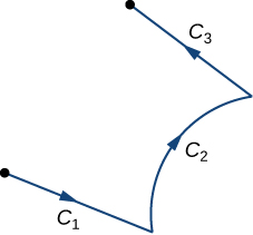
We have learned how to integrate smooth oriented curves. Now, suppose that \(C\) is an oriented curve that is not smooth, but can be written as the union of finitely many smooth curves. In this case, we say that \(C\) is a piecewise smooth curve. To be precise, curve \(C\) is piecewise smooth if \(C\) can be written as a union of n smooth curves \(C_1\), \(C_2\),…, \(C_n\) such that the endpoint of \(C_i\) is the starting point of \(C_{i+1}\) (Figure \(\PageIndex{8}\)). When curves \(C_i\) satisfy the condition that the endpoint of \(C_i\) is the starting point of \(C_{i+1}\), we write their union as \(C_1+C_2+⋯+C_n\).

Figure \(\PageIndex{8}\): The union of \(C_1\), \(C_2\), \(C_3\) is a piecewise smooth curve.

The next theorem summarizes several key properties of vector line integrals.

Theorem: Properties of Vector Line Integrals

Let \(\vecs F\) and \(\vecs G\) be continuous vector fields with domains that include the oriented smooth curve \(C\). Then

1. \(\displaystyle \int_C(\vecs F+\vecs G)·d\vecs{r}=\int_C \vecs{F} \cdot d\vecs{r}+\int_C \vecs G·d\vecs{r}\)
2. \(\displaystyle \int_C k\vecs{F} \cdot d\vecs{r}=k\int_C \vecs{F} \cdot d\vecs{r}\), where \(k\) is a constant
3. \(\displaystyle \int_{-C} \vecs{F} \cdot d\vecs{r}=-\int_{C}\vecs{F} \cdot d\vecs{r}\)
4. Suppose instead that \(C\) is a piecewise smooth curve in the domains of \(\vecs F\) and \(\vecs G\), where \(C=C_1+C_2+⋯+C_n\) and \(C_1,C_2,…,C_n\) are smooth curves such that the endpoint of \(C_i\) is the starting point of \(C_{i+1}\). Then

   \[\int_C \vecs F·d\vecs{r}=\int_{C_1} \vecs F·d\vecs{r}+\int_{C_2} \vecs F·d\vecs{r}+⋯+\int_{C_n} \vecs F·d\vecs{r}. \nonumber \]

Notice the similarities between these items and the properties of single-variable integrals. Properties i. and ii. say that line integrals are linear, which is true of single-variable integrals as well. Property iii. says that reversing the orientation of a curve changes the sign of the integral. If we think of the integral as computing the work done on a particle traveling along \(C\), then this makes sense. If the particle moves backward rather than forward, then the value of the work done has the opposite sign. This is analogous to the equation \(\displaystyle \int_a^b f(x)\,dx=−\int_b^af(x)\,dx\). Finally, if \([a_1,a_2]\), \([a_2,a_3]\),…, \([a_{n−1},a_n]\) are intervals, then

\[\int_{a_1}^{a_n}f(x) \,dx=\int_{a_1}^{a_2}f(x)\,dx+\int_{a_1}^{a_3}f(x)\,dx+⋯+\int_{a_{n−1}}^{a_n} f(x)\,dx, \nonumber \]

which is analogous to property iv.

Example \(\PageIndex{8}\): Using Properties to Compute a Vector Line Integral

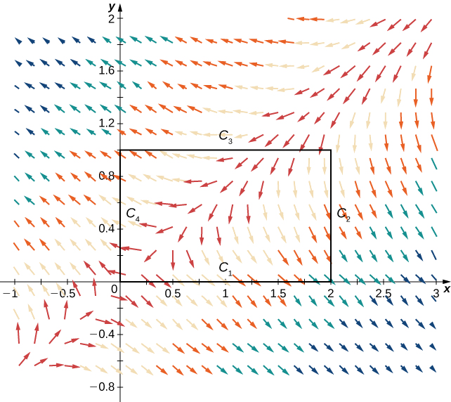
Find the value of integral \(\displaystyle \int_C \vecs F·\vecs T \,ds\), where \(C\) is the rectangle (oriented counterclockwise) in a plane with vertices \((0,0)\), \((2,0)\), \((2,1)\), and \((0,1)\), and where \(\vecs F=⟨x−2y,y−x⟩\) (Figure \(\PageIndex{9}\)).

Figure \(\PageIndex{9}\): Rectangle and vector field for Example \(\PageIndex{8}\).

Solution

Note that curve \(C\) is the union of its four sides, and each side is smooth. Therefore \(C\) is piecewise smooth. Let \(C_1\) represent the side from \((0,0)\) to \((2,0)\), let \(C_2\) represent the side from \((2,0)\) to \((2,1)\), let \(C_3\) represent the side from \((2,1)\) to \((0,1)\), and let \(C_4\) represent the side from \((0,1)\) to \((0,0)\) (Figure \(\PageIndex{9}\)). Then,

\[\int_C \vecs F·\vecs T \,dr=\int_{C_1} \vecs F·\vecs T \,dr+\int_{C_2} \vecs F·\vecs T \,dr+\int_{C_3} \vecs F·\vecs T \,dr+\int_{C_4} \vecs F·\vecs T \,dr. \nonumber \]

We want to compute each of the four integrals on the right-hand side using Equation \ref{eq12a}. Before doing this, we need a parameterization of each side of the rectangle. Here are four parameterizations (note that they traverse \(C\) counterclockwise):

\[\begin{align*} C_1&: ⟨t,0⟩,0≤t≤2\\[4pt] C_2&: ⟨2,t⟩, 0≤t≤1 \\[4pt] C_3&: ⟨2−t,1⟩, 0≤t≤2\\[4pt] C_4&: ⟨0,1−t⟩, 0≤t≤1. \end{align*}\]

Therefore,

\[\begin{align*} \int_{C_1} \vecs F·\vecs T \,dr &=\int_0^2 \vecs F(\vecs r(t))·\vecs r′(t) \,dt \\[4pt] &=\int_0^2 ⟨t−2(0),0−t⟩·⟨1,0⟩ \,dt=\int_0^2 t \,dt \\[4pt] &=\Big[\tfrac{t^2}{2}\Big]_0^2=2. \end{align*}\]

Notice that the value of this integral is positive, which should not be surprising. As we move along curve \(C_1\) from left to right, our movement flows in the general direction of the vector field itself. At any point along \(C_1\), the tangent vector to the curve and the corresponding vector in the field form an angle that is less than 90°. Therefore, the tangent vector and the force vector have a positive dot product all along \(C_1\), and the line integral will have positive value.

The calculations for the three other line integrals are done similarly:

\[\begin{align*} \int_{C_2} \vecs{F} \cdot d\vecs{r} &=\int_{0}^{1}⟨2−2t,t−2⟩·⟨0,1⟩ \,dt \\[4pt] &=\int_{0}^{1} (t−2) \,dt \\[4pt] &=\Big[\tfrac{t^2}{2}−2t\Big]_0^1=−\dfrac{3}{2}, \end{align*}\]

\[\begin{align*} \int_{C_3} \vecs F·\vecs T \,ds &=\int_0^2⟨(2−t)−2,1−(2−t)⟩·⟨−1,0⟩ \,dt \\[4pt] &=\int_0^2t \,dt=2, \end{align*}\]

and

\[\begin{align*} \int_{C_4} \vecs{F} \cdot d\vecs{r} &=\int_0^1⟨−2(1−t),1−t⟩·⟨0,−1⟩ \,dt \\[4pt] &=\int_0^1(t−1) \,dt \\[4pt] &=\Big[\tfrac{t^2}{2}−t\Big]_0^1=−\dfrac{1}{2}. \end{align*}\]

Thus, we have \(\displaystyle \int_C \vecs{F} \cdot d\vecs{r}=2\).

Exercise \(\PageIndex{8}\)

Calculate line integral \(\displaystyle \int_C \vecs{F} \cdot d\vecs{r}\), where \(\vecs F\) is vector field \(⟨y^2,2xy+1⟩\) and \(C\) is a triangle with vertices \((0,0)\), \((4,0)\), and \((0,5)\), oriented counterclockwise.

Hint

Write the triangle as a union of its three sides, then calculate three separate line integrals.

Answer

0

 

Applications of Line Integrals

Scalar line integrals have many applications. They can be used to calculate the length or mass of a wire, the surface area of a sheet of a given height, or the electric potential of a charged wire given a linear charge density. Vector line integrals are extremely useful in physics. They can be used to calculate the work done on a particle as it moves through a force field, or the flow rate of a fluid across a curve. Here, we calculate the mass of a wire using a scalar line integral and the work done by a force using a vector line integral.

Suppose that a piece of wire is modeled by curve C in space. The mass per unit length (the linear density) of the wire is a continuous function \(\rho(x,y,z)\). We can calculate the total mass of the wire using the scalar line integral \(\displaystyle \int_C \rho(x,y,z) \,ds\). The reason is that mass is density multiplied by length, and therefore the density of a small piece of the wire can be approximated by \(\rho(x^*,y^*,z^*) \,\Delta s\) for some point \((x^*,y^*,z^*)\) in the piece. Letting the length of the pieces shrink to zero with a limit yields the line integral \(\displaystyle \int_C \rho(x,y,z) \,ds\).

Example \(\PageIndex{9}\): Calculating the Mass of a Wire

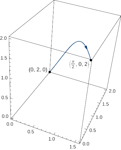
Calculate the mass of a spring in the shape of a curve parameterized by \(⟨t,2\cos t,2\sin t⟩\), \(0≤t≤\dfrac{\pi}{2}\), with a density function given by \(\rho(x,y,z)=e^x+yz\) kg/m (Figure \(\PageIndex{10}\)).

Figure \(\PageIndex{10}\): The wire from Example \(\PageIndex{9}\).

Solution

To calculate the mass of the spring, we must find the value of the scalar line integral \(\displaystyle \int_C(e^x+yz)\,ds\), where \(C\) is the given helix. To calculate this integral, we write it in terms of \(t\) using Equation \ref{eq12a}:

\[\begin{align*} \int_C \left(e^x+yz\right) \,ds &=\int_0^{\tfrac{\pi}{2}} \left((e^t+4\cos t\sin t)\sqrt{1+(−2\cos t)^2+(2\sin t)^2}\right)\,dt\\[4pt] &=\int_0^{\tfrac{\pi}{2}}\left((e^t+4\cos t\sin t)\sqrt{5}\right) \,dt \\[4pt] &=\sqrt{5}\Big[e^t+2\sin^2 t\Big]_{t=0}^{t=\pi/2}\\[4pt] &=\sqrt{5}(e^{\pi/2}+1). \end{align*}\]

Therefore, the mass is \(\sqrt{5}(e^{\pi/2}+1)\) kg.

Exercise \(\PageIndex{9}\)

Calculate the mass of a spring in the shape of a helix parameterized by \(\vecs r(t)=⟨\cos t,\sin t,t⟩\), \(0≤t≤6\pi\), with a density function given by \(\rho (x,y,z)=x+y+z\) kg/m.

Hint

Calculate the line integral of \(\rho\) over the curve with parameterization \(\vecs r\).

Answer

\(18\sqrt{2}{\pi}^2\) kg

When we first defined vector line integrals, we used the concept of work to motivate the definition. Therefore, it is not surprising that calculating the work done by a vector field representing a force is a standard use of vector line integrals. Recall that if an object moves along curve \(C\) in force field \(\vecs F\), then the work required to move the object is given by \(\displaystyle \int_C \vecs{F} \cdot d\vecs{r}\).

Example \(\PageIndex{10}\): ​​​​​​Calculating Work

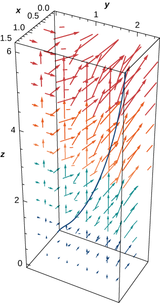
How much work is required to move an object in vector force field \(\vecs F=⟨yz,xy,xz⟩\) along path \(\vecs r(t)=⟨t^2,t,t^4⟩,\, 0≤t≤1?\) See Figure \(\PageIndex{11}\).

Solution

Let \(C\) denote the given path. We need to find the value of \(\displaystyle \int_C \vecs{F} \cdot d\vecs{r}\). To do this, we use Equation \ref{lineintformula} :

\[\begin{align*}\int_C \vecs{F} \cdot d\vecs{r} &=\int_0^1(⟨t^5,t^3,t^6⟩·⟨2t,1,4t^3⟩) \,dt \\[4pt] &=\int_0^1(2t^6+t^3+4t^9) \,dt \\[4pt] &={\Big[\dfrac{2t^7}{7}+\dfrac{t^4}{4}+\dfrac{2t^{10}}{5}\Big]}_{t=0}^{t=1}=\dfrac{131}{140}\;\text{units of work}. \end{align*}\]

Figure \(\PageIndex{11}\): The curve and vector field for Example \(\PageIndex{10}\).

 

Flux

We close this section by discussing two key concepts related to line integrals: flux across a plane curve and circulation along a plane curve. Flux is used in applications to calculate fluid flow across a curve, and the concept of circulation is important for characterizing conservative gradient fields in terms of line integrals. Both these concepts are used heavily throughout the rest of this chapter. The idea of flux is especially important for Green’s theorem, and in higher dimensions for Stokes’ theorem and the divergence theorem.

Let \(C\) be a plane curve and let \(\vecs F\) be a vector field in the plane. Imagine \(C\) is a membrane across which fluid flows, but \(C\) does not impede the flow of the fluid. In other words, \(C\) is an idealized membrane invisible to the fluid. Suppose \(\vecs F\) represents the velocity field of the fluid. How could we quantify the rate at which the fluid is crossing \(C\)?

Recall that the line integral of \(\vecs F\) along \(C\) is \(\displaystyle \int_C \vecs F·\vecs T \,ds\)—in other words, the line integral is the dot product of the vector field with the unit tangential vector with respect to arc length. If we replace the unit tangential vector with unit normal vector \(\vecs N(t)\) and instead compute integral \(\int_C \vecs F·\vecs N \,ds\), we determine the flux across \(C\). To be precise, the definition of integral \(\displaystyle \int_C \vecs F·\vecs N \,ds\) is the same as integral \(\displaystyle \int_C \vecs F·\vecs T \,ds\), except the \(\vecs T\) in the Riemann sum is replaced with \(\vecs N\). Therefore, the flux across \(C\) is defined as

\[\int_C \vecs F·\vecs N \,ds=\lim_{n\to\infty}\sum_{i=1}^{n} \vecs F(P_i^*)·\vecs N(P_i^*)\,\Delta s_i, \nonumber \]

where \(P_i^*\) and \(\Delta s_i\) are defined as they were for integral \(\displaystyle \int_C \vecs F·\vecs T \,ds\). Therefore, a flux integral is an integral that is perpendicular to a vector line integral, because \(\vecs N\) and \(\vecs T\) are perpendicular vectors.

If \(\vecs F\) is a velocity field of a fluid and \(C\) is a curve that represents a membrane, then the flux of \(\vecs F\) across \(C\) is the quantity of fluid flowing across \(C\) per unit time, or the rate of flow.

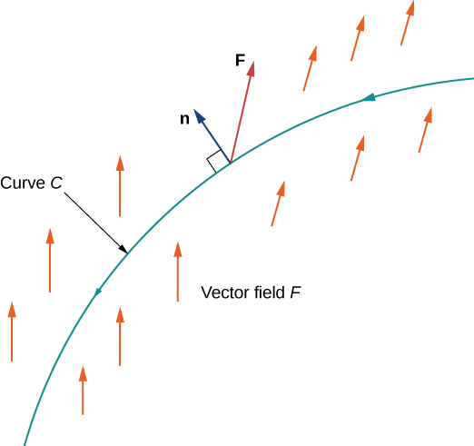
More formally, let \(C\) be a plane curve parameterized by \(\vecs r(t)=⟨x(t),\,y(t)⟩\), \(a≤t≤b\). Let \(\vecs n(t)=⟨y′(t),\,−x′(t)⟩\) be the vector that is normal to \(C\) at the endpoint of \(\vecs r(t)\) and points to the right as we traverse \(C\) in the positive direction (Figure \(\PageIndex{12}\)). Then, \(\vecs N(t)=\dfrac{\vecs n(t)}{‖\vecs n(t)‖}\) is the unit normal vector to \(C\) at the endpoint of \(\vecs r(t)\) that points to the right as we traverse \(C\).

DEFINITION: Flux

The flux of \(\vecs F\) across \(C\) is line integral

\[\int_C \vecs F·\dfrac{\vecs n(t)}{‖\vecs n(t)‖} \,ds. \nonumber \]

Figure \(\PageIndex{12}\): The flux of vector field \(\vecs F\) across curve \(C\) is computed by an integral similar to a vector line integral.

We now give a formula for calculating the flux across a curve. This formula is analogous to the formula used to calculate a vector line integral (see Equation \ref{lineintformula}).

Theorem: Calculating Flux Across a Curve

Let \(\vecs F\) be a vector field and let \(C\) be a smooth curve with parameterization \(r(t)=⟨x(t),y(t)⟩\), \(a≤t≤b\).Let \(\vecs n(t)=⟨y′(t),−x′(t)⟩\). The flux of \(\vecs F\) across \(C\) is

\[\int_C \vecs F·\vecs N\,ds=\int_a^b\vecs F(\vecs r(t))·\vecs n(t) \,dt. \label{eq84} \]

Proof

Before deriving the formula, note that

\[‖\vecs n(t)‖=‖⟨y′(t),−x′(t)⟩‖=\sqrt{{(y′(t))}^2+{(x′(t))}^2}=‖\vecs r′(t)‖. \nonumber \]

Therefore,

\[\begin{align*}\int_C \vecs F·\vecs N \,ds &=\int_C \vecs F·\dfrac{\vecs n(t)}{‖\vecs n(t)‖} \,ds \\[4pt] &=\int_a^b \vecs F·\dfrac{\vecs n(t)}{‖\vecs n(t)‖}‖\vecs r′(t)‖ \,dt \\[4pt] &=\int_a^b \vecs F(\vecs r(t))·\vecs n(t) \,dt. \end{align*}\]

\(\square\)

Example \(\PageIndex{11}\): Flux across a Curve

Calculate the flux of \(\vecs F=⟨2x,2y⟩\) across a unit circle oriented counterclockwise (Figure \(\PageIndex{13}\)).

Figure \(\PageIndex{13}\): A unit circle in vector field \(\vecs F=⟨2x,\,2y⟩\).

Solution

To compute the flux, we first need a parameterization of the unit circle. We can use the standard parameterization \(\vecs r(t)=⟨\cos t,\sin t⟩\), \(0≤t≤2\pi\). The normal vector to a unit circle is \(⟨\cos t,\sin t⟩\). Therefore, the flux is

\[\begin{align*} \int_C \vecs F·\vecs N \,ds &=\int_0^{2\pi}⟨2\cos t,2\sin t⟩·⟨\cos t,\sin t⟩ \,dt\\[4pt] &=\int_0^{2\pi}(2{\cos}^2t+2{\sin}^2t) \,dt \\[4pt] &=2\int_0^{2\pi}({\cos}^2t+{\sin}^2t) \,dt \\[4pt] &=2\int_0^{2\pi} \,dt=4\pi.\end{align*}\]

Exercise \(\PageIndex{11}\)

Calculate the flux of \(\vecs F=⟨x+y,2y⟩\) across the line segment from \((0,0)\) to \((2,3)\), where the curve is oriented from left to right.

Hint

Use Equation \ref{eq84}.

Answer

\(3/2\)

Let \(\vecs F(x,y)=⟨P(x,y),Q(x,y)⟩\) be a two-dimensional vector field. Recall that integral \(\displaystyle \int_C \vecs F·\vecs T \,ds\) is sometimes written as \(\displaystyle \int_C P\,dx+Q\,dy\). Analogously, flux \(\displaystyle \int_C \vecs F·\vecs N \,ds\) is sometimes written in the notation \(\displaystyle \int_C −Q\,dx+P\,dy\), because the unit normal vector \(\vecs N\) is perpendicular to the unit tangent \(\vecs T\). Rotating the vector \(d\vecs{r}=⟨dx,dy⟩\) by 90° results in vector \(⟨dy,−dx⟩\). Therefore, the line integral in Example \(\PageIndex{8}\) can be written as \(\displaystyle \int_C −2y\,dx+2x\,dy\).

 

Circulation

Now that we have defined flux, we can turn our attention to circulation. The line integral of vector field \(\vecs F\) along an oriented closed curve is called the circulation of \(\vecs F\) along \(C\). Circulation line integrals have their own notation: \(\oint_C \vecs F·\vecs T \,ds\). The circle on the integral symbol denotes that \(C\) is “circular” in that it has no endpoints. Example \(\PageIndex{5}\) shows a calculation of circulation.

To see where the term circulation comes from and what it measures, let \(\vecs v\) represent the velocity field of a fluid and let \(C\) be an oriented closed curve. At a particular point \(P\), the closer the direction of \(\vecs v(P)\) is to the direction of \(\vecs T(P)\), the larger the value of the dot product \(\vecs v(P)·\vecs T(P)\). The maximum value of \(\vecs v(P)·\vecs T(P)\) occurs when the two vectors are pointing in the exact same direction; the minimum value of \(\vecs v(P)·\vecs T(P)\) occurs when the two vectors are pointing in opposite directions. Thus, the value of the circulation \(\oint_C \vecs v·\vecs T \,ds\) measures the tendency of the fluid to move in the direction of \(C\).

Example \(\PageIndex{12}\): Calculating Circulation

Let \(\vecs F=⟨−y,\,x⟩\) be the vector field from Example \(\PageIndex{3}\) and let \(C\) represent the unit circle oriented counterclockwise. Calculate the circulation of \(\vecs F\) along \(C\).

Solution

We use the standard parameterization of the unit circle: \(\vecs r(t)=⟨\cos t,\sin t⟩\), \(0≤t≤2\pi\). Then, \(\vecs F(\vecs r(t))=⟨−\sin t,\cos t⟩\) and \(\vecs r′(t)=⟨−\sin t,\cos t⟩\). Therefore, the circulation of \(\vecs F\) along \(C\) is

\[\begin{align*} \oint_C \vecs F·\vecs T \,ds &=\int_0^{2\pi}⟨−\sin t,\cos t⟩·⟨−\sin t,\cos t⟩ \,dt \\[4pt] &=\int_0^{2\pi} ({\sin}^2 t+{\cos}^2 t) \,dt \\[4pt] &=\int_0^{2\pi} \,dt=2\pi \;\text{units of work}. \end{align*}\]

Notice that the circulation is positive. The reason for this is that the orientation of \(C\) “flows” with the direction of \(\vecs F\). At any point along the circle, the tangent vector and the vector from \(\vecs F\) form an angle of less than 90°, and therefore the corresponding dot product is positive.

In Example \(\PageIndex{12}\), what if we had oriented the unit circle clockwise? We denote the unit circle oriented clockwise by \(−C\). Then

\[\oint_{−C} \vecs F·\vecs T \,ds=−\oint_C \vecs F·\vecs T \,ds=−2\pi \;\text{units of work}. \nonumber \]

Notice that the circulation is negative in this case. The reason for this is that the orientation of the curve flows against the direction of \(\vecs F\).

Exercise \(\PageIndex{12}\)

Calculate the circulation of \(\vecs F(x,y)=⟨−\dfrac{y}{x^2+y^2},\,\dfrac{x}{x^2+y^2}⟩\) along a unit circle oriented counterclockwise.

Hint

Use Equation \ref{eq84}.

Answer

\(2\pi\) units of work

Example \(\PageIndex{13}\): Calculating Work

Calculate the work done on a particle that traverses circle \(C\) of radius 2 centered at the origin, oriented counterclockwise, by field \(\vecs F(x,y)=⟨−2,\,y⟩\). Assume the particle starts its movement at \((1,\,0)\).

Solution

The work done by \(\vecs F\) on the particle is the circulation of \(\vecs F\) along \(C\): \(\oint_C \vecs F·\vecs T \,ds\). We use the parameterization \(\vecs r(t)=⟨2\cos t,\,2\sin t⟩\), \(0≤t≤2\pi\) for \(C\). Then, \(\vecs r′(t)=⟨−2\sin t,\,2\cos t⟩\) and \(\vecs F(\vecs r(t))=⟨−2,\,2\sin t⟩\). Therefore, the circulation of \(\vecs F\) along \(C\) is

\[\begin{align*} \oint_C \vecs F·\vecs T \,ds &=\int_0^{2\pi} ⟨−2,2\sin t⟩·⟨−2\sin t,2\cos t⟩ \,dt\\[4pt] &=\int_0^{2\pi} (4\sin t+4\sin t\cos t) \,dt\\[4pt] &={\Big[−4\cos t+4{\sin}^2 t\Big]}_0^{2\pi}\\[4pt] &=\left(−4\cos(2\pi)+2{\sin}^2(2\pi)\right)−\left(−4\cos(0)+4{\sin}^2(0)\right)\\[4pt] &=−4+4=0\;\text{units of work}.\end{align*}\]

The force field does zero work on the particle.

Notice that the circulation of \(\vecs F\) along \(C\) is zero. Furthermore, notice that since \(\vecs F\) is the gradient of \(f(x,y)=−2x+\dfrac{y^2}{2}\), \(\vecs F\) is conservative. We prove in a later section that under certain broad conditions, the circulation of a conservative vector field along a closed curve is zero.

Exercise \(\PageIndex{14}\)

Calculate the work done by field \(\vecs F(x,y)=⟨2x,\,3y⟩\) on a particle that traverses the unit circle. Assume the particle begins its movement at \((−1,\,0)\).

Hint

Use Equation \ref{eq84}.

Answer

\(0\) units of work

 

Key Concepts

• Line integrals generalize the notion of a single-variable integral to higher dimensions. The domain of integration in a single-variable integral is a line segment along the \(x\)-axis, but the domain of integration in a line integral is a curve in a plane or in space.
• If \(C\) is a curve, then the length of \(C\) is \(\displaystyle \int_C \,ds\).
• There are two kinds of line integral: scalar line integrals and vector line integrals. Scalar line integrals can be used to calculate the mass of a wire; vector line integrals can be used to calculate the work done on a particle traveling through a field.
• Scalar line integrals can be calculated using Equation \ref{eq12a}; vector line integrals can be calculated using Equation \ref{lineintformula}.
• Two key concepts expressed in terms of line integrals are flux and circulation. Flux measures the rate that a field crosses a given line; circulation measures the tendency of a field to move in the same direction as a given closed curve.

 

Key Equations

• Calculating a scalar line integral
  \(\displaystyle \int_C f(x,y,z) \,ds=\int_a^bf(\vecs r(t))\sqrt{{(x′(t))}^2+{(y′(t))}^2+{(z′(t))}^2} \,dt\)
• Calculating a vector line integral
  \(\displaystyle \int_C \vecs F·d\vecs{r}=\int_C \vecs F·\vecs T \,ds=\int_a^b\vecs F(\vecs r(t))·\vecs r′(t)\,dt\)
  or
  \(\displaystyle \int_C P\,dx+Q\,dy+R\,dz=\int_a^b \left(P\big(\vecs r(t)\big)\dfrac{dx}{dt}+Q\big(\vecs r(t)\big)\dfrac{dy}{dt}+R\big(\vecs r(t)\big)\dfrac{dz}{dt}\right) \,dt\)
• Calculating flux
  \(\displaystyle \int_C \vecs F·\dfrac{\vecs n(t)}{‖\vecs n(t)‖}\,ds=\int_a^b \vecs F(\vecs r(t))·\vecs n(t) \,dt\)

 

Glossary

circulation

the tendency of a fluid to move in the direction of curve \(C\). If \(C\) is a closed curve, then the circulation of \(\vecs F\) along \(C\) is line integral \(∫_C \vecs F·\vecs T \,ds\), which we also denote \(∮_C\vecs F·\vecs T \,ds\).

closed curve

a curve for which there exists a parameterization \(\vecs r(t), a≤t≤b\), such that \(\vecs r(a)=\vecs r(b)\), and the curve is traversed exactly once

flux

the rate of a fluid flowing across a curve in a vector field; the flux of vector field \(\vecs F\) across plane curve \(C\) is line integral \(∫_C \vecs F·\frac{\vecs n(t)}{‖\vecs n(t)‖} \,ds\)

line integral

the integral of a function along a curve in a plane or in space

orientation of a curve

the orientation of a curve \(C\) is a specified direction of \(C\)

piecewise smooth curve

an oriented curve that is not smooth, but can be written as the union of finitely many smooth curves

scalar line integral

the scalar line integral of a function \(f\) along a curve \(C\) with respect to arc length is the integral \(\displaystyle \int_C f\,ds\), it is the integral of a scalar function \(f\) along a curve in a plane or in space; such an integral is defined in terms of a Riemann sum, as is a single-variable integral

vector line integral

the vector line integral of vector field \(\vecs F\) along curve \(C\) is the integral of the dot product of \(\vecs F\) with unit tangent vector \(\vecs T\) of \(C\) with respect to arc length, \(∫_C \vecs F·\vecs T\, ds\); such an integral is defined in terms of a Riemann sum, similar to a single-variable integral