2.1: Limits and Continuity

Limit

In the last section, we saw that as the interval over which we calculated got smaller, the secant slopes approached the tangent slope. The limit gives us better language with which to discuss the idea of “approaches.”

The limit of a function describes the behavior of the function when the variable is near, but does not equal, a specified number (see the figure below).

Limit

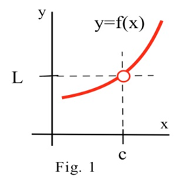
If the values of \(f(x)\) get closer and closer, as close as we want, to one number \(L\) as we take values of \(x\) very close to (but not equal to) a number \(c\), then we say "the limit of \(f(x)\) as \(x\) approaches \(c\) is \(L\)" and we write \[\lim\limits_{x\to c} f(x)=\mathbf{L}.\nonumber \] The symbol "\( \to \)" means "approaches" or, less formally, "gets very close to".

(This definition of the limit isn't stated as formally as it could be, but it is sufficient for our purposes in this course.)

Note:

• \(\bf f(c)\) is a single number that describes the behavior (value) of \(f(x)\) AT the point \(x = c\).
• \(\lim\limits_{x\to c} f(x)\) is a single number that describes the behavior of \(f(x)\) NEAR, BUT NOT AT, the point \(x = c\).

If we have a graph of the function near \(x = c\), then it is usually easy to determine \( \lim\limits_{x\to c} f(x) \).

(Here is a link to the pictures used in the following video as well as elsewhere in this chapter: Graphs for Limits and Continuity Examples.)

Example \(\PageIndex{1}\)

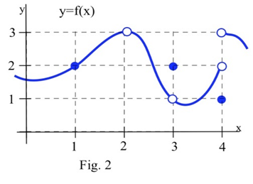
Use the graph of \(y = f(x)\) in the figure below to determine the following limits:

1. \(\lim\limits_{x\to 1} f(x)\)
2. \(\lim\limits_{x\to 2} f(x)\)
3. \(\lim\limits_{x\to 3} f(x)\)
4. \(\lim\limits_{x\to 4} f(x)\)

Solution

1. \[\lim_{x \to 1} f(x) = 2\nonumber\]When \(x\) is very close to 1, the values of \(f(x)\) are very close to \(y = 2\). In this example, it happens that \(f(1) = 2\), but that is irrelevant for the limit. The only thing that matters is what happens for \(x\) close to 1 but \(x \neq 1\).
2. \(f(2)\) is undefined, but we only care about the behavior of \(f(x)\) for \(x\) close to 2 but not equal to 2. When \(x\) is close to 2, the values of \(f(x)\) are close to 3. If we restrict \(x\) close enough to 2, the values of \(y\) will be as close to 3 as we want, so \( \lim\limits_{x\to 2} f(x) = 3 \).
3. When \(x\) is close to 3 (or "as \(x\) approaches the value 3"), the values of \(f(x)\) are close to 1 (or "approach the value 1"), so \( \lim\limits_{x\to 3} f(x) = 1 \). For this limit it is completely irrelevant that \(f(3) = 2\), We only care about what happens to \(f(x)\) for \(x\) close to and not equal to 3.
4. This one is harder and we need to be careful. When \(x\) is close to 4 and slightly less than 4 (\(x\) is just to the left of 4 on the \(x\)-axis), then the values of \(f(x)\) are close to 2. But if \(x\) is close to 4 and slightly larger than 4 then the values of \(f(x)\) are close to 3. If we only know that \(x\) is very close to 4, then we cannot say whether \(y = f(x)\) will be close to 2 or close to 3 – it depends on whether \(x\) is on the right or the left side of 4. In this situation, the \(f(x)\) values are not close to a single number so we say \(\lim\limits_{x\to 4} f(x)\) does not exist. It is irrelevant that \(f(4) = 1\). The limit, as \(x\) approaches 4, would still be undefined if \(f(4)\) was 3 or 2 or anything else.

We can also explore limits using tables and using algebra.

Example \(\PageIndex{2}\)

Find \( \lim\limits_{x\to 1} \dfrac{2x^2-x-1}{x-1} \).

Solution

You might try to evaluate \(f(x) = \frac{2x^2-x-1}{x-1}\) at \(x = 1\), but \(f(x)\) is not defined at \(x = 1\). It is tempting, but wrong, to conclude that this function does not have a limit as \(x\) approaches 1.

Using tables: Trying some "test" values for \(x\) which get closer and closer to 1 from both the left and the right, we get

\( x \)	\( f(x) \)
0.9	2.82
0.9998	2.9996
0.999994	2.999988
0.9999999	2.9999998
\( \to 1 \)	\( \to 3 \)

\( x \)	\( f(x) \)
1.1	3.2
1.003	3.006
1.0001	3.0002
1.000007	3.000014
\( \to 1 \)	\( \to 3 \)

The function \(f\) is not defined at \(x = 1\), but when \(x\) is close to 1, the values of \(f(x)\) are getting very close to 3. We can get \(f(x)\) as close to 3 as we want by taking \(x\) very close to 1 so \[\lim\limits_{x\to 1} \dfrac{2x^2-x-1}{x-1}=3.\nonumber \]

Using algebra: We could have found the same result by noting that \[ f(x)= \dfrac{2x^2-x-1}{x-1} = \dfrac{(2x+1)(x-1)}{(x-1)} = 2x+1\nonumber \] as long as \(x \neq 1\). (If \(x\neq 1\), then \(x–1 \neq 0\) so it is valid to divide the numerator and denominator by the factor \(x–1\).) The "\(x\to 1\)" part of the limit means that \(x\) is close to 1 but not equal to 1, so our division step is valid and \[ \lim\limits_{x\to 1}\dfrac{2x^2-x-1}{x-1} = \lim\limits_{x\to 1} 2x+1 = 3,\nonumber \] which is our answer.

Using a graph: We can graph \( y=f(x)= \dfrac{2x^2-x-1}{x-1} \) for \(x\) close to 1:

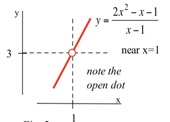
Notice that whenever \(x\) is close to 1, the values of \(y = f(x)\) are close to 3. Since \(f\) is not defined at \(x = 1\), the graph has a hole above \(x = 1\), but we only care about what \(f(x)\) is doing for \(x\) close to but not equal to 1.

Example \(\PageIndex{3}\)

Find \(\lim \limits_{x\to 3} \dfrac{\frac{1}{x} -\frac{1}{3} }{x-3}\).

Solution

Notice that this function is not defined at \(x = 3\). We can find the limit using algebra. Giving the two terms in the numerator a common denominator, we can simplify:

\[ \frac{\frac{1}{x} -\frac{1}{3} }{x-3} = \frac{\frac{1}{x} \cdot \frac{3}{3} -\frac{1}{3} \cdot \frac{x}{x} }{x-3} = \frac{\frac{3}{3x} -\frac{x}{3x} }{x-3} =\frac{\frac{3-x}{3x} }{x-3} \nonumber \]

Remember that dividing a fraction is the same as multiplying by the reciprocal, so
\[\frac{\frac{3-x}{3x} }{x-3} =\frac{\frac{3-x}{3x} }{\frac{x-3}{1} }\nonumber \] is equivalent to \[\frac{3-x}{3x} \cdot \frac{1}{x-3}\nonumber \]

To simplify further, we need to factor a negative 1 out of the numerator. Then we can cancel the term \(\left(x-3\right)\)
\(\dfrac{-1(x-3)}{3x} \cdot \dfrac{1}{x-3} =\dfrac{-1}{3x}\) as long as \(x \neq 3\)

Now we can evaluate the limit using this simplified form.
\[\lim\limits_{x\to 3} \frac{\frac{1}{x} -\frac{1}{3} }{x-3} = \lim\limits_{x\to 3} \frac{-1}{3x} = -\frac{1}{9} \nonumber \]

One Sided Limits

Sometimes, what happens to us at a place depends on the direction we use to approach that place. If we approach Niagara Falls from the upstream side, then we will be 182 feet higher and have different worries than if we approach from the downstream side. Similarly, the values of a function near a point may depend on the direction we use to approach that point.

Left and Right Limits

The left limit of \(f(x)\) as \(x\) approaches \(c\) is \(L\) if the values of \(f(x)\) get as close to \(L\) as we want when \(x\) is very close to and left of \(c\) (i.e., \(x \lt \mathbf{c}\)). We write \[\lim\limits_{x\to c^-} f(x)=L.\nonumber \]

The right limit of \(f(x)\) as \(x\) approaches \(c\), written with \(\bf x \to c^+\), is \(L\) if the values of \(f(x)\) get as close to \(L\) as we want when \(x\) is very close to and right of \(c\) (i.e., \(x \gt \mathbf{c}\)). We write \[\lim\limits_{x\to c^+} f(x)=L.\nonumber \]

Example \(\PageIndex{4}\)

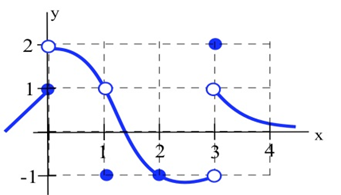
Evaluate the one sided limits of the function \(f(x)\) graphed below at \(x = 0\) and \(x = 1\).

Solution

As \(x\) approach 0 from the left, the value of the function is getting closer to 1, so \( \lim\limits_{x\to 0^-} f(x) = 1. \)

As \(x\) approaches 0 from the right, the value of the function is getting closer to 2, so \( \lim\limits_{x\to 0^+} f(x) = 2. \)

Notice that since the limit from the left and limit from the right are different, the general limit, \( \lim\limits_{x\to 0} f(x) \), does not exit.

At \(x\) approaches 1 from either direction, the value of the function is approaching 1, so \[\lim\limits_{x\to 1^-} f(x) = \lim\limits_{x\to 1^+} f(x) = \lim\limits_{x\to 1} f(x) = 1. \nonumber \]

Continuity

A function that is "friendly" and doesn’t have any breaks or jumps in it is called continuous. More formally,

Continuity at a Point

A function \(\bf f\) is continuous at \(\bf x = a \) if and only if \( \lim\limits_{x\to a} \mathbf{f(x)} = \mathbf{f(a)}\).

The graph below illustrates some of the different ways a function can behave at and near a point, and the table contains some numerical information about the function and its behavior.

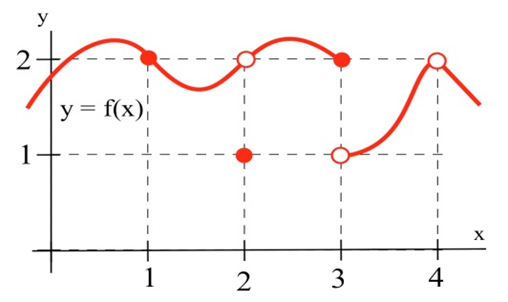
\( a \)	\( f(a) \)	\( \lim\limits_{x\to a} f(x) \)
1	2	2
2	1	2
3	2	Does not exist (DNE)
4	Undefined	2

Based on the information in the table, we can conclude that \(f\) is continuous at 1 since \( \lim\limits_{x\to 1} f(x) = 2 = f(1)\).

We can also conclude from the information in the table that \(f\) is not continuous at 2 or 3 or 4, because \( \lim\limits_{x\to 2} f(x) \neq f(2) \), \( \lim\limits_{x\to 3} f(x) \neq f(3) \), and \( \lim\limits_{x\to 4} f(x) \neq f(4) \).

The behaviors at \(x = 2\) and \(x = 4\) exhibit a hole in the graph, sometimes called a removable discontinuity, since the graph could be made continuous by changing the value of a single point. The behavior at \( x = 3 \) is called a jump discontinuity, since the graph jumps between two values.

So which functions are continuous? It turns out pretty much every function you’ve studied is continuous where it is defined: polynomial, radical, rational, exponential, and logarithmic functions are all continuous where they are defined. Moreover, any combination of continuous functions is also continuous.

This is helpful, because the definition of continuity says that for a continuous function, \( \lim\limits_{x\to a} f(x) = f(a) \). That means for a continuous function, we can find the limit by direct substitution (evaluating the function) if the function is continuous at \(a\).

Example \(\PageIndex{5}\)

Evaluate using continuity, if possible:

1. \( \lim\limits_{x\to 2} x^3-4x \)
2. \( \lim\limits_{x\to 2} \dfrac{x-4}{x+3} \)
3. \( \lim\limits_{x\to 2} \dfrac{x-4}{x-2} \)

Solution

1. The given function is polynomial, and is defined for all values of \(x\), so we can find the limit by direct substitution:\[ \lim\limits_{x\to 2} x^3-4x = 2^3-4(2) = 0. \nonumber \]
2. The given function is rational. It is not defined at \(x = -3\), but we are taking the limit as \(x\) approaches 2, and the function is defined at that point, so we can use direct substitution:\[ \lim\limits_{x\to 2} \dfrac{x-4}{x+3} = \dfrac{2-4}{2+3}= -\dfrac{2}{5}. \nonumber \]
3. This function is not defined at \(x = 2\), and so is not continuous at \(x = 2\). We cannot use direct substitution.