2.10: Other Applications

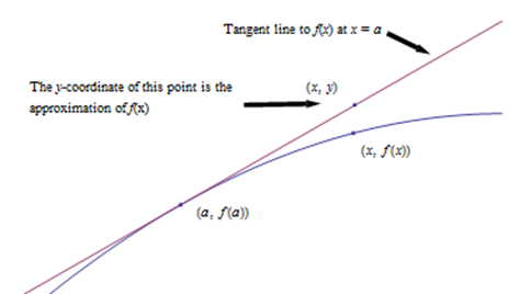
Tangent Line Approximation

Back when we first thought about the derivative, we used the slope of secant lines over tiny intervals to approximate the derivative:

\[f'(a) \cong \frac{\Delta y}{\Delta x} = \frac{f(x) - f(a)}{x-a} \nonumber\]

Now that we have other ways to find derivatives, we can exploit this approximation to go the other way. Solve the expression above for \(f(x)\), and you’ll get the tangent line approximation:

The Tangent Line approximation (TLA)

To approximate the value of \(f(x)\) using TLA, find some \(a\) where

1. \(a\) and \(x\) are “close,” and
2. You know the exact values of both \(f (a)\) and \(f ‘(a)\). Then \[f(x) \cong f(a) + f'(a)(x-a).\nonumber\]

Another way to look at the same formula:

\[\Delta y \cong f'(a) \Delta x\nonumber\]

How close is close? It depends on the shape of the graph of \(f\). In general, the closer the better.

Example \(\PageIndex{1}\)

Suppose we know that \(g(20) = 5\) and \(g’(20) = 1.4\). Use this information to approximate \(g(23)\) and \(g(18)\).

Solution

Using the tangent line approximation:

\(g(23) \approx 5 + (1.4)(23 – 20) = 9.2\)

\(g(18) \approx 5 + (1.4)(18 – 20) = 2.2\)

Note that we don’t know if these approximations are close – but they’re the best we can do with the limited information we have to start with. Note also that 18 and 23 are sort of close to 20, so we can hope these approximations are pretty good. We’d feel more confident using this information to approximate \(g(20.003)\). We’d feel very unsure using this information to approximate \(g(55)\).

Elasticity

We know that demand functions are decreasing, so when the price increases, the quantity demanded goes down. But what about revenue = price \( \times \) quantity? When the price increases will revenue go down because the demand dropped so much? Or will revenue increase because demand didn't drop very much?

Example \(\PageIndex{2}\)

Suppose a company's demand function is \(D(p) = 100 - p^2\), and the company's current price is $5. What will happen to revenue if they raise the price $0.05?

Solution

We are more interested in how the price change compares to the demand change, so we are going to convert everything to relative (percent) changes.

The price has increased by \[\frac{\Delta p}{p} = \frac{\$0.05}{\$5} = 0.01 = 1\%\nonumber \]

The demand decreased from \(D(5) = 100-5^2 = 75\) to \(D(5.05) = 100-5.05^2 = 74.4975\), a total change of \(75-74.4975 = -0.5025\). As a relative change, that's \[\frac{\Delta q}{q} = \frac{-0.05025}{75} = -0.0067 = -0.67\%\nonumber \]

By raising the price 1%, the demand only fell by 0.67%. Since the price is increasing more than the demand falls, we would expect total revenue to increase. In this case we say that the demand is inelastic.

Elasticity of demand is a measure of how demand reacts to price changes. It's normalized – that means the particular prices and quantities don't matter, and everything is treated as a percent change.

Following the logic of the example above, we want to compare the relative change in demand to the relative change in price, or in other words, we want to look at \[\frac{\frac{\Delta q}{q}}{\frac{\Delta p}{p}}.\nonumber \] By approximating the changes in demand and price by the derivatives, this formula simplifies to \[\frac{\frac{dq}{q}}{\frac{dp}{p}} = \frac{p}{q}\cdot\frac{dq}{dp}\nonumber \]

Elasticity of Demand

Given a demand function that gives \(q\) in terms of \(p\), so \(q = D(p)\), the elasticity of demand is \[E=\left|\frac{p}{q}\cdot \frac{dq}{dp}\right| = \left|\frac{p}{q}\cdot D'(p)\right| \nonumber \]

(Note that since demand is a decreasing function of \(p\), the derivative is negative. That's why we have the absolute values – so \(E\) will always be positive.)

You may also see this formula written as \[E = - \frac{p \cdot D'(p)}{D(p)}\nonumber \] The two forms of the equation are equivalent, and you can use either.

• If \(E \lt 1\), we say demand is inelastic. In this case, raising prices increases revenue.
• If \(E \gt 1\), we say demand is elastic. In this case, raising prices decreases revenue.
• If \(E = 1\), we say demand is unitary. \(E = 1\) at critical points of the revenue function.

Interpretation of elasticity

If the price increases by 1%, the demand will decrease by E%.

Example \(\PageIndex{3}\)

A company sells \( q \) ribbon winders per year at $\( p \) per ribbon winder. The demand function for ribbon winders is given by \( p=300-0.02q \). Find the elasticity of demand when the price is $70 apiece. Will an increase in price lead to an increase in revenue?

Solution

First, we need to solve the demand equation so it gives \( q \) in terms of \( p \), so that we can find \( \frac{dq}{dp} \): \( p=300-0.02q \), so \( q=15000-50p \). Then \( \frac{dq}{dp}=-50 \).

We need to find \( q \) when \( p = 70 \): \[ q = 11500. \nonumber \]

Now compute \[ E=\left| \frac{p}{q}\cdot\frac{dq}{dp} \right|=\left| \frac{70}{11500}\cdot(-50) \right| \approx 0.3 \nonumber \]

\(E \lt 1\), so demand is inelastic. Increasing the price by 1% would only cause a 0.3% drop in demand. Increasing the price would lead to an increase in revenue, so it seems that the company should increase its price.

The demand for products that people have to buy, such as onions, tends to be inelastic. Even if the price goes up, people still have to buy about the same amount of onions, and revenue will not go down. The demand for products that people can do without, or put off buying, such as cars, tends to be elastic. If the price goes up, people will just not buy cars right now, and revenue will drop.

Example \(\PageIndex{4}\)

A company finds the demand \( q \), in thousands, for their kites to be \( q=400-p^2 \) at a price of \( p \) dollars. Find the elasticity of demand when the price is $5 and when the price is $15. Then find the price that will maximize revenue.

Solution

Calculating the derivative, \( \frac{dq}{dp}=-2p \). The elasticity equation as a function of \( p \) will be: \[ E=\left| \frac{p}{q}\cdot\frac{dq}{dp} \right|=\left| \frac{p}{400-p^2}\cdot (-2p) \right| =\left| \frac{-2p^2}{400-p^2} \right| \nonumber \]

Evaluating this to find the elasticity at $5 and at $15:

\[ E(5) = \left| \frac{-2(5)^2}{400-(5)^2} \right| \approx 0.133 \nonumber \] So the demand is inelastic when the price is $5.

At a price of $5, a 1% increase in price would decrease demand by only 0.133%. Revenue could be raised by increasing prices.

\[ E(15) = \left| \frac{-2(15)^2}{400-(15)^2} \right| \approx 2.571 \nonumber \] So the demand is elastic when the price is $15.

At a price of $15, a 1% increase in price would decrease demand by 2.571%. Revenue could be raised by decreasing prices.

To maximize the revenue, we could solve for when \( E = 1 \): \[ \begin{align*} \left| \frac{-2p^2}{400-p^2} \right| & = 1 \\ 2p^2 & = 400-p^2 \\ 3p^2 & = 400 \\ p & = \sqrt{\frac{400}{3}}\approx 11.55. \end{align*} \nonumber \]

A price of $11.55 will maximize the revenue.

As you saw the in last example, elasticity provides another way to determine the price that will maximize revenue given a demand function. It is not quicker or easier than the methods learned earlier in the course, but you are welcome to use either technique.