8.2: The Cumulative Distribution Function

To recap the previous section, we defined what is meant by a random variable. A random variable, \(X\), is a function from \(S \rightarrow \mathbb{R} \). Afterwards, we then discussed the probability mass function, \(f\), associated to the random variable \(X\).

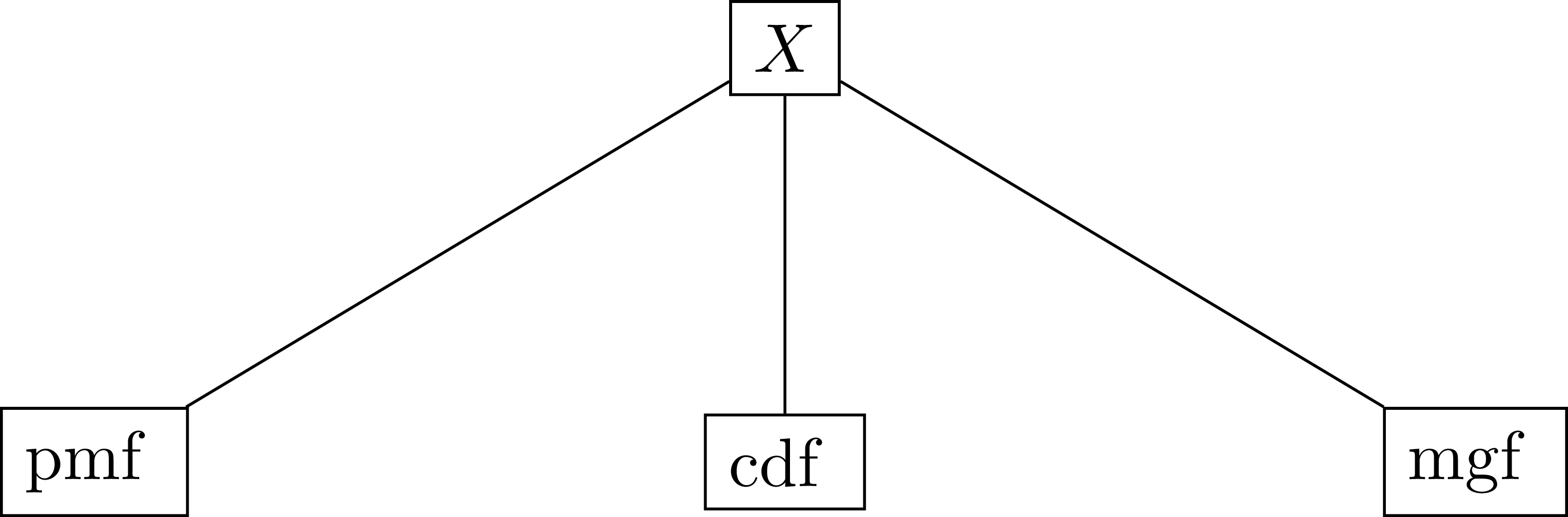
Note that \(X\), itself, is a function and associated with this function is the probability mass function. In total, there are three important functions associated with a discrete random variable. These functions are

1) the probability mass function (pmf)

2) the cumulative distribution function (cdf)

3) the moment generating function (mgf)

In this section, we will discuss the cumulative distribution function.

Definition: Cumulative Distribution Function

Definition: For a discrete random variable \(X\) with probability mass function \(f\), we define the cumulative distribution function (c.d.f.) of \(X\), often denoted by \(F\), to be:

\[ F(x) = P(X \leq x), ~~ - \infty < x < \infty \nonumber \]

As a quick comparison, allow us to discuss the difference between a pmf and a cdf. As we recall from the previous section, the job of a pmf is to tell us the probability that \(X\) equals a single, particular value. Meanwhile, a cdf tells us the probability that \(X\) is less than or equal to a particular value.

Example \(\PageIndex{1}\)

Suppose a random variable \(X\) has the following probability mass function.

\( f(x) = P(X = x) =
\begin{cases}
.855, & \mbox{if } x = 0 \\
.140, & \mbox{if } x = 100000 \\ .005 , & \mbox{if } x = 200000 \\ 0, & \mbox{otherwise}
\end{cases}\)

Find the cumulative distribution function of \(X\).

Answer 1

One way to find the cumulative distribution function is to evaluate the cdf at selected points and then generalize our findings. This method can be extremely inefficient, especially if there are many possible values for \(X\). However, this is a good exercise to do at least once since this will give some intuition about how the cumulative distribution function behaves aand so we perform this method here. Allow us to find the following: \(F(-100), F(-1), F(-0.01), F(0), F(0.01), F(1), F(50,000), F(99,999.99), F(100,000), F(100,000.01), F(150,000), F(199,999.99)\), \(F(200,000) \), \( F(1,000,000) \). To do so, we will use the third part of the theorem from the previous section.

1. \( F(-100) = P(X \leq -100) = \sum_{\text{all} x \leq -100} f(x) = 0 \)

2. \( F(-1) = P(X \leq -1) = 0 \sum_{\text{all} x \leq -1} f(x) = 0 \)

3. \( F(-0.01) = P(X \leq -0.01) = \sum_{\text{all} x \leq -0.01} f(x) = 0 \)

4. \( F(0) = P(X \leq 0) = 0 \sum_{\text{all} x \leq 0} f(x) = f(0) = 0.855 \)

5. \( F(1) = P(X \leq 1) = 0 \sum_{\text{all} x \leq 1} f(x) = f(0) = 0.855 \)

6. \( F(50,000) = P(X \leq 50,000) = 0 \sum_{\text{all} x \leq 50,000} f(x) = f(0) = 0.855 \)

7. \( F(99,999.99) = P(X \leq 99,999.99) = 0 \sum_{\text{all} x \leq 99,999.99} f(x) = f(0) = 0.855 \)

8. \( F(100,000) = P(X \leq 100,000) = 0 \sum_{\text{all} x \leq 100,000} f(x) = f(0) + f(100,000) = 0.855 + 0.140 = 0.995 \)

9. \( F(100,000.01) = P(X \leq 100,000.01) = 0 \sum_{\text{all} x \leq 100,000.01} f(x) = f(0) + f(100,000) = 0.855 + 0.140 = 0.995 \)

10. \( F(150,000) = P(X \leq 150,000) = 0 \sum_{\text{all} x \leq 150,000} f(x) = f(0) + f(100,000) = 0.855 + 0.140 = 0.995 \)

11. \( F(199,999.99) = P(X \leq 199,999.99) = 0 \sum_{\text{all} x \leq 199,999.99} f(x) = f(0) + f(100,000) = 0.855 + 0.140 = 0.995 \)

12. \( F(200,000) = P(X \leq 200,000) = 0 \sum_{\text{all} x \leq 200,000} f(x) = f(0) + f(100,000) + f(200,000) = 0.855 + 0.140 + 0.005 = 1 \)

13. \( F(1,000,000) = P(X \leq 1,000,000) = 0 \sum_{\text{all} x \leq 1,000,000} f(x) = f(0) + f(100,000) + f(200,000) = 0.855 + 0.140 + 0.005 = 1 \)

Based off these computations, we see that for any value \( x < 0\), the cdf is zero.

At \(x=0\), the cdf is equal to 0.855.

For any \(x\) where \(0 \leq x < 100,000\) the cdf should also be equal to 0.855 since the only possible value of \(X\) that occurs with a nonzero probability is at \(X = 0 \).

At \(x=100,000\), the cdf is equal to 0.995.

For any \(x\) where \(100,000 \leq x < 200,000\) the cdf should also be equal to 0.995 since the only possible values of \(X\) that occurs with a nonzero probability is at \(X = 0 \) and \(X = 100,000 \).

At \(x=200,000\), the cdf is equal to 1.

For any \(x\) where \(x \geq 200,00 \) the cdf should also be equal to 1 since the possible values of \(X\) that occurs with a nonzero probability is at \(X = 0 \), \(X = 100,000 \), and \(X = 200,000 \).

Putting everything together, we see that

\( F(x) = P(X \leq x) =
\begin{cases}
0, & \mbox{if } x < 0 \\ 0.855, & \mbox{if } 0 \leq x < 100,000 \\ .995, & \mbox{if } 100,000 \leq x < 200,000 \\
1, & \mbox{if } x \geq 200000
\end{cases}\)

Answer 2

More efficiently, we may use the following remark.

Note

If \(X\) is a discrete random variables whose possible values are \(x_1, x_2, \ldots, x_n \) where \( x_1 < x_2 < \ldots < x_n \), then the cumulative distribution function of \(X\) is a step function that starts off at a "height" of zero, "ends" at a height of 1, and whose jump at \(x_i\) is equal to \(f(x_i)\).

To use this remark, allow us to graph the pmf. Doing so yields the following image:

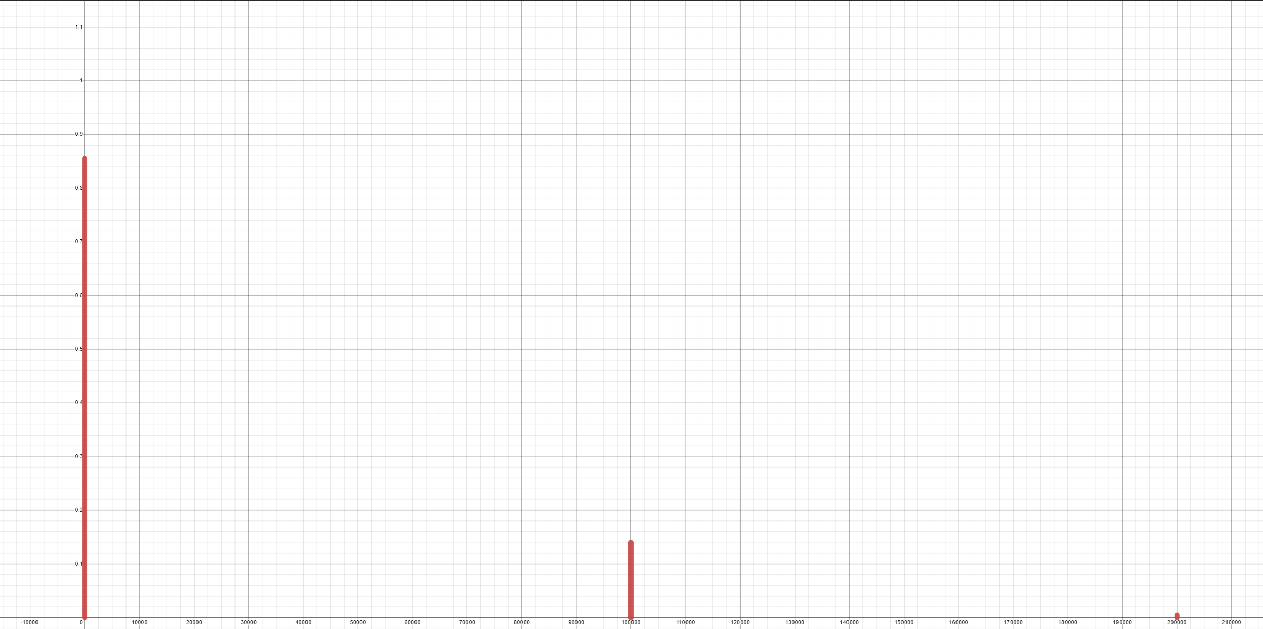
Based off our remark, the cumulative distribution function will be a step function that starts at a height of zero, ends at a height of 1, and whose jump in between will occur at each possible value of \(X\). The height of this jump is precisely the height of each red bar.

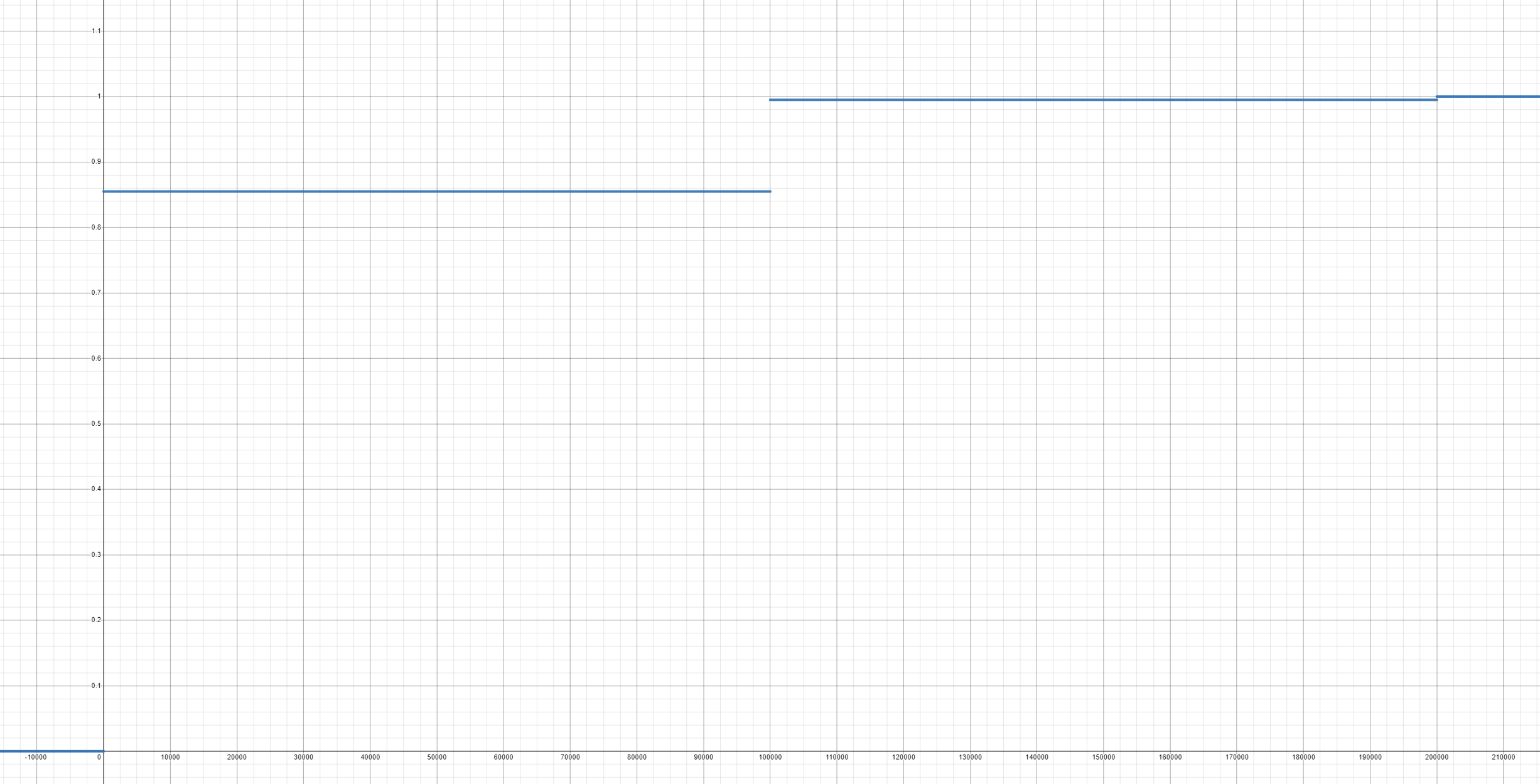
Looking at the graph, we see that \( F(x) = P(X \leq x) =
\begin{cases}
0, & \mbox{if } x < 0 \\ 0.855, & \mbox{if } 0 \leq x < 100,000 \\ .995, & \mbox{if } 100,000 \leq x < 200,000 \\
1, & \mbox{if } x \geq 200000
\end{cases}\)