8.3: Expected Values

Now that we are familiar with random variables, we are going to discuss a natural idea - the average of a random variable. In fact, we argue that the average of a random variable is something that we all are already familiar with. Consider the following question:

Motivating Example 1 \(\PageIndex{1}\)

Suppose for a certain college course, the grading policy is the following:

1. Quiz Average - 15%
2. Exam 1 - 20%
3. Exam 2 - 20%
4. Exam 3 - 20%
5. Final Exam - 25%

Let us suppose your quiz average is an 85, your Exam 1 score is 72, your Exam 2 score is 85, your Exam 3 score is 90 and your Final Exam score is 81. How would you compute your average?

Answer

We take every score and multiply the score by the "weight". We then add the resulting products to compute our average for the class. Doing so yields, \( \text{Average} = 0.15(85) + 0.2(72) + 0.2(85) + 0.2(90) + 0.25(81) = 82.4 \) and so you have obtained a \(B-\) in the course.

Allow us to now introduce some notation. In the above example, we can denote our score on any assignment as \(x_i\) and the corresponding weight outlined in the grading policy can be thought of as \(f(x_i)\). Hence, we obtain the following table:

Assignment	\(x_i\)	\(f(x_i)\)	\( x_i f(x_i) \)
Quiz Average	0.15	85	0.15(85)
Exam 1	0.20	72	0.2(72)
Exam 2	0.20	85	0.2(85)
Exam 3	0.20	90	0.2(90)
Final Exam	0.25	81	0.25(81)

We see that the average is computed by adding up the entries under the column labeled \( x_i f(x_i) \). Hence, we see that

\[ \text{Average} = \sum_{i=1}^{5} x_i f(x_i) \nonumber \]

And if we were to generalize the above formula, we can conclude that

\[ \text{Average} = \sum_{ \text{all} ~ x} x f(x) \]

The above equation is how we precisely define the average of a discrete random variable.

Definition: Expected Value

Definition: For a discrete random variable \(X\) with probability mass function \(f\), we define the expected (average) value of \(X\), denoted by \( \mathbb{E}[X] \) or by \( \mu \), to be \[ \mathbb{E}[X] = \sum_{ \text{all} ~ x} x f(x) \nonumber \]

Allow us to take a look at a few computations involving the expected value of a random variable.

Example 2 \(\PageIndex{1}\)

Suppose the probability mass function of \(X\) is given by \( f(x) = P(X = x) =
\begin{cases}
.855, & \mbox{if } x = 0 \\
.140, & \mbox{if } x = 100000 \\ .005 , & \mbox{if } x = 200000 \\ 0, & \mbox{otherwise}
\end{cases}\)

Find \( \mathbb{E}[X] \).

Answer

To find the average of \(X\), we simply apply the formula, \( \text{Average} = \sum_{ \text{all} ~ x} x f(x) \). That is, we multiply each value of the random variable by its "weight" and add up the products. Doing so yields the following result:

\begin{align*} \mathbb{E}[X] &= \sum_{\text{all} ~ x} x f(x) \\ &= 0(0.855) + 100,000(0.140) + 200,000(0.005) \\ &= 15,000 \end{align*}

Example 3 \(\PageIndex{1}\)

Suppose \(X\) is a discrete random variable whose probability mass function is given by \( f(x) = P(X = x) =
\begin{cases}
cx, & \mbox{if } x = 1, 2, 3, 4 \\ 0, & \mbox{otherwise}
\end{cases}\)

where \(c\) denotes some constant.

1) Find the value of \(c\).

2) Find \( \mathbb{E}[X] \).

Answer

1) First note that \(c\) cannot be any arbitrary real number. For instance, if we said that \( c = 2 \) then we are saying that \( P(X = 4) = f(4) = 8 \) and so we have violated our theorems since we proved a probability cannot be greater than 1.

For questions like these, there is only one, unique value for \(c\). To find the appropriate value of \(c\), we use the third property of a probability mass function. Since \( \sum_{\text{all} ~ x } f(x) = 1 \), then we obtain the following:

\begin{align*} \sum_{\text{all} ~ x } f(x) &= 1 \\ \sum_{\text{all} ~ x } cx &= 1 \\ 1c + 2c + 3c + 4c &= 1 \\ 10c &= 1 \\ x &= \frac{1}{10} \end{align*}

And so \( c = \frac{1}{10} \).

2) We now know that \(X\) has the following probability mass function:

\( f(x) = P(X = x) =
\begin{cases}
\frac{x}{10}, & \mbox{if } x = 1, 2, 3, 4 \\ 0, & \mbox{otherwise}
\end{cases}\)

To find \( \mathbb{E}[X] \), we simply apply our definition. Doing so yields:

\begin{align*} \mathbb{E}[X] &= \sum_{\text{all} ~ x} x f(x) \\ &= \sum_{x = 1}^{4} x \frac{x}{10} \\ =& \sum_{x = 1}^{4} \frac{x^2}{10} \\ &= \frac{1^2}{10} + \frac{2^2}{10} + \frac{3^2}{10} + \frac{4^2}{10} \\ &= \frac{30}{10} \\ &= 3 \end{align*}

Example 4 \(\PageIndex{1}\)

Suppose the probability mass function of \(X\) is given by \( f(x) = P(X = x) =
\begin{cases}
\frac{1}{6}, & \mbox{if } x = 1, 2, 3, 4, 5, 6 \\
0, & \mbox{otherwise}
\end{cases}\)

Find \( \mathbb{E}[X] \).

Answer

To find the average of \(X\), we simply apply the formula, \( \text{Average} = \sum_{ \text{all} ~ x} x f(x) \). That is, we multiply each value of the random variable by its "weight" and add up the products. Doing so yields the following result:

\begin{align*} \mathbb{E}[X] &= \sum_{\text{all} ~ x} x f(x) \\ &= \frac{1}{6}(1) + \frac{1}{6}(2) + \frac{1}{6}(3) + \frac{1}{6}(4) + \frac{1}{6}(5) + \frac{1}{6}(6) \\ &= \frac{1}{6} (1 + 2 + 3 + 4 + 5 + 6) \\ &= 3.5 \end{align*}

There are two important remarks to make concerning \( \mathbb{E}[X] \).

Remarks

1) First note that the average value is not guaranteed to be a possible value of \(X\). In our motivating question, the average was an 82.4, yet we never scored an 82.4 on any of the assignments. The same can be said about the two examples considered above. Notice in Example 2, the average was 15,000 which is not a possible value of \(X\) and in Example 3 the average was 3.5 which is again not a possible value of \(X\).

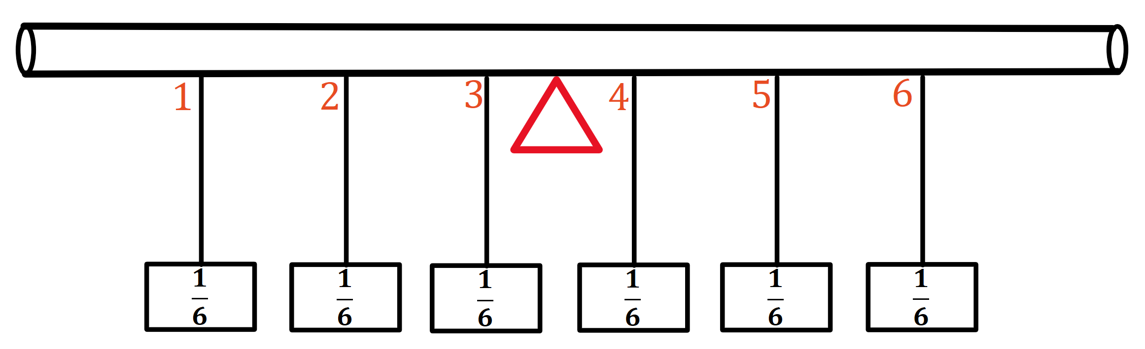
2) From physics, especially classical mechanics, there is a nice way to interpret the expected value. The expected value of a discrete random variable is nothing more than the so called "center of mass" or "balance point". What do we mean by this? \\

Suppose \(X\) is a discrete random variable with values \(x_i\) and corresponding probabilities \(p_i\). Imagine a weightless rod such that at location \(x_i\) on the rod, an object of weight \(p_i\) is placed. The point at which the rod balances is precisely \( \mathbb{E}[X] \).

For instance, consider the following bar graph for the last problem.

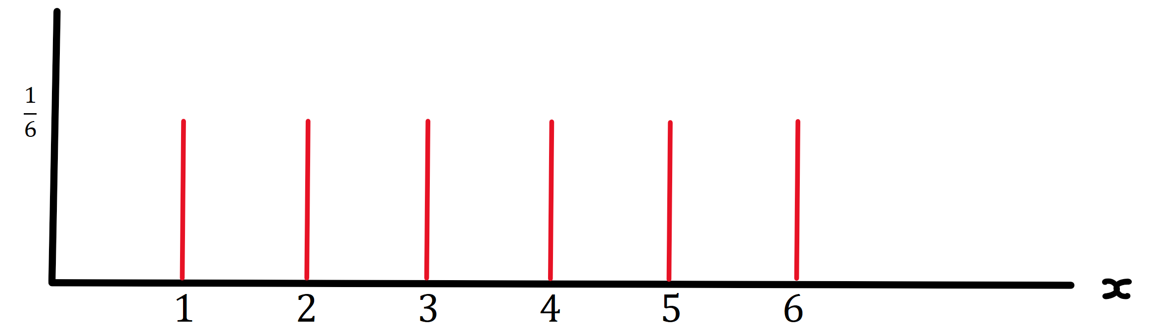
Imagine the \(x\)-axis as a weightless rod and at each 1 unit interval, we attach a weight of \( \frac{1}{6} \) pounds.

Where would you have to place your finger to balance this rod on top of? Precisely at the half way mark which is at \( \mathbb{E}[X]= 3.5\).

In summary, to find the average of a discrete random variable \(X\), we simply compute \( \sum_{\text{all} ~ x} x f(x) \). Note that in order to do so, we require the probability mass function of \(X\). Hence, at this point, to find the average of a discrete random variable, we need the probability mass function of the random variable.

The question we will now consider for the remainder of this section is the following: given a random variable \(X\), we know how to compute \( \mathbb{E}[X] \). However, what if we wish to compute the average of a function of \(X\)?

For instance, suppose we defined some random variable \(X\). Instead of computing \( \mathbb{E}[X] \), we might be interested in computing \( \mathbb{E}[X^2] \) or \( \mathbb{E}[5x^3] \).

More formally, the question we are considering is given a random variable \(X\) and a real valued function \(g\), how can we find \( \mathbb{E}[g(X)] \)? Note that \(g(X)\) is a new random variable which we will denote by \(Y\) and there are two ways in which we can compute the average of \(g(X) = Y \).

Method 1 to Compute \( \mathbb{E}[u(X)] \).

Recall we stated that at this point, to find the average of a discrete random variable, we need the probability mass function of the random variable. Hence, given a random variable \(X\), if we wish to find the average of \(g(X) = Y \), it suffices to derive the probability mass function of \(Y\) and use the probability mass function to find the average.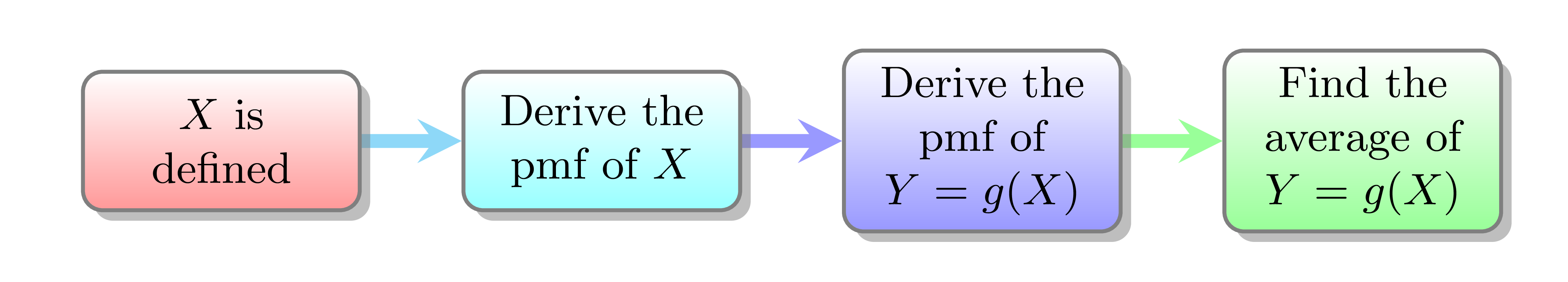

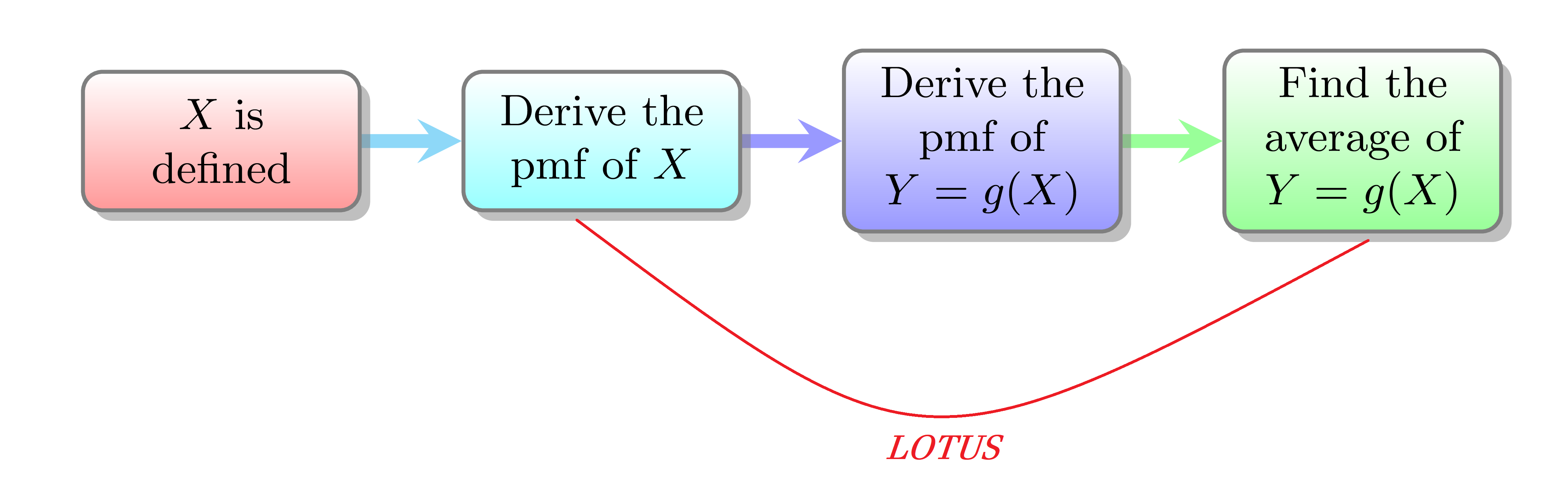
In practice, the above process can be somewhat difficult and so allow us to introduce Method 2 which is an important theorem.

Method 2 to Compute \( \mathbb{E}[u(X)] \).

Theorem: The Law of the Unconscious Statistician \(\PageIndex{1}\)

Theorem: If \(X\) is a discrete random variable with probability mass function \(f\) and if \(u(X)\) is any real-valued function of \(X\), then

\[ \mathbb{E}[u(X)] = \sum_{\text{all} ~ x} u(x) f(x) \]

We will see that applying The Law of the Unconscious Statistician (The LOTUS), allows us to skip the derivation of the probability mass function of \( u(X) = Y \).

Example 5 \(\PageIndex{1}\)

Suppose \(X\) is a discrete random variable whose probability mass function is given by \( f(x) = P(X = x) =
\begin{cases}
0.2, & \mbox{if } x = -1 \\
0.5, & \mbox{if } x = 0 \\ 0.3 , & \mbox{if } x = 1 \\ 0, & \mbox{otherwise}
\end{cases}\)

Find \( \mathbb{E}[X^2] \).

Method 1

Looking back at the flowchart presented under Method 1, we see that the random variable \(X\) has been defined and the probability mass function of \(X\) has already been given. Thus, we now must derive the probability mass function of \(Y\) which we will denote by \(g\). Recall how to derive a probability mass function. We first ask ourselves, what are the possible values of \(Y\)? Seeing the \(X : -1, 0 1 \) then \(Y = X^2: 1, 0, 1 \). So \( Y: 0, 1 \). We now must find the probabilities that \(Y\) takes each value. Note that

\( P(Y = 0) = P(X^2 = 0) = P(X=0) = f(0) = 0.5 \).

\( P(Y = 1) = P(X^2 = 1) = P( \{X = -1\} \cup \{ X = 1\}) = P( \{X = -1\}) + P( \{ X = 1\}) = f(0) + f(1) = 0.2 + 0.3 = 0.5 \).

Summarizing everything in a function, we see that \( g(y) = P(Y = y) =
\begin{cases}
0.5, & \mbox{if } x = 0 \\
0.5, & \mbox{if } x = 1 \\ 0, & \mbox{otherwise}
\end{cases}\)

Hence,

\( \matbb{E}[Y] = \sum_{\text{all} ~ y} y g(y) = 0(0.5) + 1(0.5) = 0.5 \).

Method 2

Alternatively, we may apply The LOTUS. Recall The LOTUS states \[ \mathbb{E}[u(X)] = \sum_{\text{all} ~ x} u(x) f(x) \]

Hence \begin{align*} \mathbb{E}[X^2] &= \sum_{\text{all} ~ x} x^2 f(x) \] \\ &= (-1)^2 f(-1) + 0^2 f(0) + 1^2 f(1) \\ &= f(-1) + f(1) \\ &= 0.2 + 0.3 \\ &=0.5 \end{align*}

Observe that Method 1 could become a complicated process if the original random variable has many values and if \(u(X)\) is not injective whereas Method 2 simply relies on the underlying probability mass function of the random variable in the transformation.

Example 6 \(\PageIndex{1}\)

Suppose \(X\) is a discrete random variable whose probability mass function is given by \( f(x) = P(X = x) =
\begin{cases}
\frac{x}{10}, & \mbox{if } x = 1, 2, 3, 4 \\ 0, & \mbox{otherwise}
\end{cases}\)

Find \( \mathbb{E}[X^2] \).

Answer

To find \( \mathbb{E}[X^2] \), we apply The LOTUS. Doing so yields:

\begin{align*} \mathbb{E}[X^2] &= \sum_{\text{all} ~ x} x^2 f(x) \\ &= \sum_{x = 1}^{4} x^2 \frac{x}{10} \\ \sum_{x = 1}^{4} \frac{x^3}{10} \\ &= \frac{1^3}{10} + \frac{2^3}{10} + \frac{3^3}{10} + \frac{4^3}{10} \\ &= \frac{100}{10} \\ &= 10. \end{align*}

Theorem \(\PageIndex{1}\)

Theorem: Suppose \(X\) is a discrete random variable. Then the following hold:

1) If \(c\) is a constant, then \( \mathbb{E}[c] = c \).

2) If \(c\) is a constant, and \( u \) is a real-valued function of \(X\) then \( \mathbb{E}[c u(X)] = c \mathbb{E}[u(X)] \).

3) If \(a\) and \(b\) are constants, then \( \mathbb{E}[aX + b] = a \mathbb{E}[X] + b\).

4) If \(u\) and \(v\) are real-valued functions of \(X\), then \( \mathbb{E}[u(X) + v(X)] = \mathbb{E}[u(X)] + \mathbb{E}[v(X)] \).

5) If \(a\) and \(b\) are constants and \(u\) and \(v\) are real-valued functions of \(X\), then \( \mathbb{E}[au(X) + bv(X)] = a \mathbb{E}[u(X)] + b \mathbb{E}[v(X)] \).

Here is an application of the above theorem.

Example 7 \(\PageIndex{1}\)

Suppose \(X\) is a discrete random variable whose probability mass function is given by \( f(x) = P(X = x) =
\begin{cases}
\frac{x}{10}, & \mbox{if } x = 1, 2, 3, 4 \\ 0, & \mbox{otherwise}
\end{cases}\)

Find \( \mathbb{E}[X(5-X)] \).

Answer

Although we can apply The LOTUS to the above problem, allow us to use the preceding theorem. Doing so yields:

\begin{align*} \mathbb{E}[X(5-X)] &= \mathbb{E}[5X - X^2] \\ &= \mathbb{E}[5X] - \mathbb{E}[X^2] \\ &= 5 \mathbb{E}[X] - \mathbb{E}[X^2] \\ &= 5(3) - 10 \\ &= 5. \end{align*}

To conclude this section, we present a definition which will be important in the next lecture.

Definition: The \(n^{th} \) Moment

Definition: Let \(n\) denote a positive integer and suppose \(X\) is a random variable. We refer to \( \mathbb{E} [X^n] \) sd the \( n^{th} \) moment of \(X\).

This means \( \mathbb{E}[X] \) is the first moment of \(X\) and \( \mathbb{E}[X^2] \) is the second moment of \(X\) and so on and so forth.