8.3: Polar Coordinates

Plotting Points Using Polar Coordinates

When we think about plotting points in the plane, we usually think of rectangular coordinates \((x,y)\) in the Cartesian coordinate plane. However, there are other ways of writing a coordinate pair and other types of grid systems. In this section, we introduce to polar coordinates, which are points labeled \((r,\theta)\) and plotted on a polar grid. The polar grid is represented as a series of concentric circles radiating out from the pole, or the origin of the coordinate plane.

The polar grid is scaled as the unit circle with the positive \(x\)-axis now viewed as the polar axis and the origin as the pole. The first coordinate \(r\) is the radius or length of the directed line segment from the pole. The angle \(\theta\), measured in radians, indicates the direction of \(r\). We move counterclockwise from the polar axis by an angle of \(\theta\),and measure a directed line segment the length of \(r\) in the direction of \(\theta\). Even though we measure \(\theta\) first and then \(r\), the polar point is written with the \(r\)-coordinate first. For example, to plot the point \(\left(2,\dfrac{\pi}{4}\right)\),we would move \(\dfrac{\pi}{4}\) units in the counterclockwise direction and then a length of \(2\) from the pole. This point is plotted on the grid in Figure \(\PageIndex{2}\).

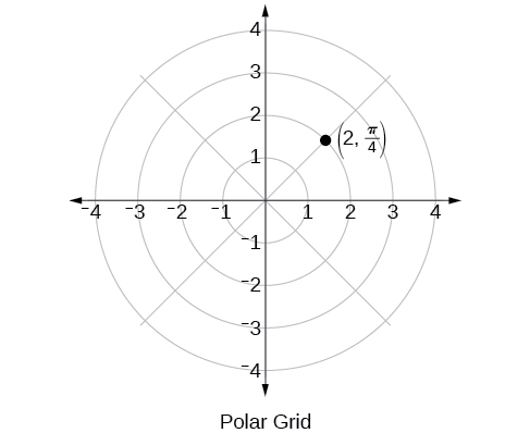
Figure \(\PageIndex{2}\)

Example \(\PageIndex{1}\): Plotting a Point on the Polar Grid

Plot the point \(\left(3,\dfrac{\pi}{2}\right)\) on the polar grid.

Solution

The angle \(\dfrac{\pi}{2}\) is found by sweeping in a counterclockwise direction \(90°\) from the polar axis. The point is located at a length of \(3\) units from the pole in the \(\dfrac{\pi}{2}\) direction, as shown in Figure \(\PageIndex{3}\).

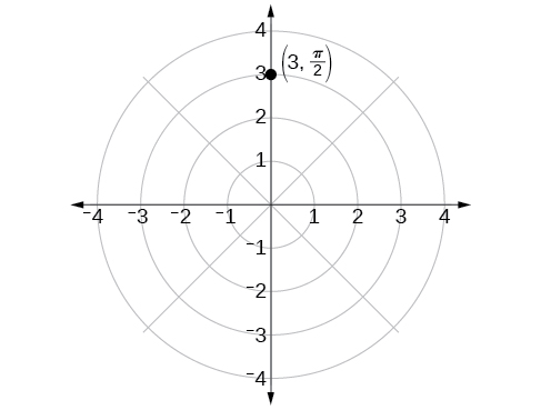
Figure \(\PageIndex{3}\)

Converting from Rectangular Coordinates to Polar Coordinates

To convert rectangular coordinates to polar coordinates, we will use two other familiar relationships. With this conversion, however, we need to be aware that a set of rectangular coordinates will yield more than one polar point.

CONVERTING FROM RECTANGULAR COORDINATES TO POLAR COORDINATES

Converting from rectangular coordinates to polar coordinates requires the use of one or more of the relationships illustrated in Figure \(\PageIndex{10}\).

\(\cos \theta=\dfrac{x}{r}\) or \(x=r \cos \theta\)

\(\sin \theta=\dfrac{y}{r}\) or \(y=r \sin \theta\)

\(r^2=x^2+y^2\)

\(\tan \theta=\dfrac{y}{x}\)

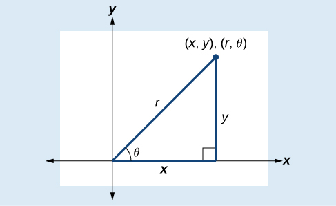
Figure \(\PageIndex{10}\)

Example \(\PageIndex{4}\): Writing Rectangular Coordinates as Polar Coordinates

Convert the rectangular coordinates \((3,3)\) to polar coordinates.

Solution

We see that the original point \((3,3)\) is in the first quadrant. To find \(\theta\), use the formula \(\tan \theta=\dfrac{y}{x}\). This gives

\[\begin{align*} \tan \theta&= \dfrac{3}{3}\\ \tan \theta&= 1\\ {\tan}^{-1}(1)&= \dfrac{\pi}{4} \end{align*}\]

To find \(r\), we substitute the values for \(x\) and \(y\) into the formula \(r=\sqrt{x^2+y^2}\). We know that \(r\) must be positive, as \(\dfrac{\pi}{4}\) is in the first quadrant. Thus

\[\begin{align*} r&= \sqrt{3^2+3^2}\\ r&= \sqrt{9+9}\\ r&= \sqrt{18}\\ &= 3\sqrt{2} \end{align*}\]

So, \(r=3\sqrt{2}\) and \(\theta=\dfrac{\pi}{4}\), giving us the polar point \((3\sqrt{2},\dfrac{\pi}{4})\). See Figure \(\PageIndex{11}\).

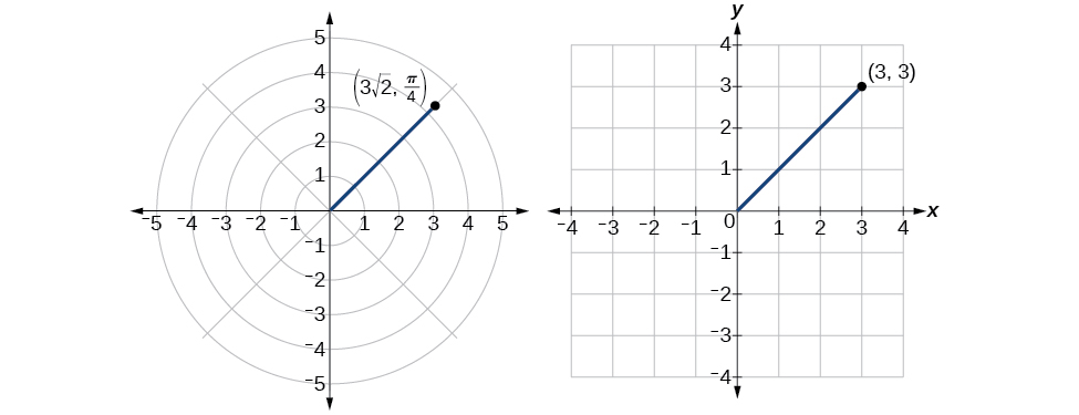
Figure \(\PageIndex{11}\)

Analysis

There are other sets of polar coordinates that will be the same as our first solution. For example, the points \(\left(−3\sqrt{2}, \dfrac{5\pi}{4}\right)\) and \(\left(3\sqrt{2},−\dfrac{7\pi}{4}\right)\) will coincide with the original solution of \(\left(3\sqrt{2}, \dfrac{\pi}{4}\right)\). The point \(\left(−3\sqrt{2}, \dfrac{5\pi}{4}\right)\) indicates a move further counterclockwise by \(\pi\), which is directly opposite \(\dfrac{\pi}{4}\). The radius is expressed as \(−3\sqrt{2}\). However, the angle \(\dfrac{5\pi}{4}\) is located in the third quadrant and, as \(r\) is negative, we extend the directed line segment in the opposite direction, into the first quadrant. This is the same point as \(\left(3\sqrt{2}, \dfrac{\pi}{4}\right)\). The point \(\left(3\sqrt{2}, −\dfrac{7\pi}{4}\right)\) is a move further clockwise by \(−\dfrac{7\pi}{4}\), from \(\dfrac{\pi}{4}\). The radius, \(3\sqrt{2}\), is the same.

Transforming Equations between Polar and Rectangular Forms

We can now convert coordinates between polar and rectangular form. Converting equations can be more difficult, but it can be beneficial to be able to convert between the two forms. Since there are a number of polar equations that cannot be expressed clearly in Cartesian form, and vice versa, we can use the same procedures we used to convert points between the coordinate systems. We can then use a graphing calculator to graph either the rectangular form or the polar form of the equation.

How to: Given an equation in polar form, graph it using a graphing calculator

1. Change the MODE to POL, representing polar form.
2. Press the Y= button to bring up a screen allowing the input of six equations: \(r_1\), \(r_2\),..., \(r_6\).
3. Enter the polar equation, set equal to \(r\).
4. Press GRAPH.

Example \(\PageIndex{5A}\): Writing a Cartesian Equation in Polar Form

Write the Cartesian equation \(x^2+y^2=9\) in polar form.

Solution

The goal is to eliminate \(x\) and \(y\) from the equation and introduce \(r\) and \(\theta\). Ideally, we would write the equation \(r\) as a function of \(\theta\). To obtain the polar form, we will use the relationships between \((x,y)\) and \((r,\theta)\). Since \(x=r \cos \theta\) and \(y=r \sin \theta\), we can substitute and solve for \(r\).

\(\begin{align*} {(r \cos \theta)}^2+{(r \sin \theta)}^2&= 9\\ r^2 {\cos}^2 \theta+r^2 {\sin}^2 \theta&= 9\\ r^2({\cos}^2 \theta+{\sin}^2 \theta)&= 9\\ r^2(1)&= 9\qquad \text {Substitute } {\cos}^2 \theta+{\sin}^2 \theta=1\\ r&= \pm 3\qquad \text {Use the square root property.} \end{align*}\)

Thus, \(x^2+y^2=9\),\(r=3\),and \(r=−3\) should generate the same graph. See Figure \(\PageIndex{12}\).

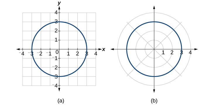
Figure \(\PageIndex{12}\): (a) Cartesian form \(x^2+y^2=9\) (b) Polar form \(r=3\)

To graph a circle in rectangular form, we must first solve for \(y\).

\[\begin{align*} x^2+y^2&= 9\\ y^2&= 9-x^2\\ y&= \pm \sqrt{9-x^2} \end{align*}\]

Note that this is two separate functions, since a circle fails the vertical line test. Therefore, we need to enter the positive and negative square roots into the calculator separately, as two equations in the form \(Y_1=\sqrt{9−x^2}\) and \(Y_2=−\sqrt{9−x^2}\). Press GRAPH.