8.4: Polar Coordinates - Graphs

Testing Polar Equations for Symmetry

Just as a rectangular equation such as \(y=x^2\) describes the relationship between \(x\) and \(y\) on a Cartesian grid, a polar equation describes a relationship between \(r\) and \(\theta\) on a polar grid. Recall that the coordinate pair \((r,\theta)\) indicates that we move counterclockwise from the polar axis (positive \(x\)-axis) by an angle of \(\theta\), and extend a ray from the pole (origin) \(r\) units in the direction of \(\theta\). All points that satisfy the polar equation are on the graph.

Symmetry is a property that helps us recognize and plot the graph of any equation. If an equation has a graph that is symmetric with respect to an axis, it means that if we folded the graph in half over that axis, the portion of the graph on one side would coincide with the portion on the other side. By performing three tests, we will see how to apply the properties of symmetry to polar equations. Further, we will use symmetry (in addition to plotting key points, zeros, and maximums of \(r\)) to determine the graph of a polar equation.

In the first test, we consider symmetry with respect to the line \(\theta=\dfrac{\pi}{2}\) (\(y\)-axis). We replace \((r,\theta)\) with \((−r,−\theta)\) to determine if the new equation is equivalent to the original equation. For example, suppose we are given the equation \(r=2 \sin \theta\);

\[\begin{align*} r&= 2 \sin \theta \\ -r&= 2 \sin -\theta \qquad \text{Replace } (r,\theta) \text{ with }(-r,-\theta). \\ -r&= -2 \sin \theta \qquad \text{Identity: }\sin(-\theta)=-\sin \theta. \\ r&= 2 \sin \theta \qquad \text{Multiply both sides by }-1 \end{align*}\]

This equation exhibits symmetry with respect to the line \(\theta=\dfrac{\pi}{2}\).

In the second test, we consider symmetry with respect to the polar axis (\(x\)-axis). We replace \((r,\theta)\) with \((r,−\theta)\) or \((−r,\pi−\theta)\) to determine equivalency between the tested equation and the original. For example, suppose we are given the equation \(r=1−2 \cos \theta\).

\[\begin{align*} r&= 1-2 \cos \theta \\ r&= 1-2 \cos(-\theta)\qquad \text{Replace }(r,\theta) \text{ with }(r,-\theta). \\ r&= 1-2 \cos \theta \qquad \text{Even/Odd identity} \end{align*}\]

The graph of this equation exhibits symmetry with respect to the polar axis.

In the third test, we consider symmetry with respect to the pole (origin). We replace \((r,\theta)\) with \((−r,\theta)\) to determine if the tested equation is equivalent to the original equation. For example, suppose we are given the equation \(r=2 \sin(3\theta)\).

\(r=2 \sin(3\theta)\)

\(−r=2 \sin(3\theta)\)

The equation has failed the symmetry test, but that does not mean that it is not symmetric with respect to the pole. Passing one or more of the symmetry tests verifies that symmetry will be exhibited in a graph. However, failing the symmetry tests does not necessarily indicate that a graph will not be symmetric about the line \(\theta=\dfrac{\pi}{2}\), the polar axis, or the pole. In these instances, we can confirm that symmetry exists by plotting reflecting points across the apparent axis of symmetry or the pole. Testing for symmetry is a technique that simplifies the graphing of polar equations, but its application is not perfect.

Note: SYMMETRY TESTS

A polar equation describes a curve on the polar grid. The graph of a polar equation can be evaluated for three types of symmetry, as shown in Figure \(\PageIndex{2}\).

Figure \(\PageIndex{2}\): (a) A graph is symmetric with respect to the line \(\theta=\dfrac{\pi}{2}\) (y-axis) if replacing \((r,\theta)\) with \((−r,−\theta)\) yields an equivalent equation. (b) A graph is symmetric with respect to the polar axis (x-axis) if replacing \((r,\theta)\) with \((r,−\theta)\) or \((−r,\pi−\theta)\) yields an equivalent equation. (c) A graph is symmetric with respect to the pole (origin) if replacing \((r,\theta)\) with \((−r,\theta)\) yields an equivalent equation.

How to: Given a polar equation, test for symmetry.

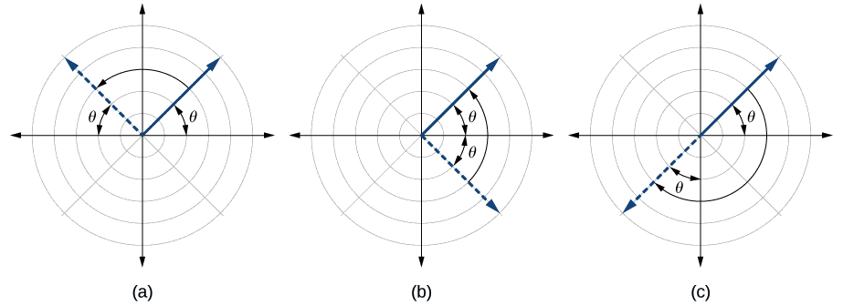
1. Substitute the appropriate combination of components for \((r,\theta)\): \((−r,−\theta)\) for \(\theta=\dfrac{\pi}{2}\) symmetry; \((r,−\theta)\) for polar axis symmetry; and \((−r,\theta)\) for symmetry with respect to the pole.
2. If the resulting equations are equivalent in one or more of the tests, the graph produces the expected symmetry.

Graphing Polar Equations by Plotting Points

To graph in the rectangular coordinate system we construct a table of \(x\) and \(y\) values. To graph in the polar coordinate system we construct a table of \(\theta\) and \(r\) values. We enter values of \(\theta\) into a polar equation and calculate \(r\). However, using the properties of symmetry and finding key values of \(\theta\) and \(r\) means fewer calculations will be needed.

Finding Zeros and Maxima

To find the zeros of a polar equation, we solve for the values of \(\theta\) that result in \(r=0\). Recall that, to find the zeros of polynomial functions, we set the equation equal to zero and then solve for \(x\). We use the same process for polar equations. Set \(r=0\), and solve for \(\theta\).

For many of the forms we will encounter, the maximum value of a polar equation is found by substituting those values of \(\theta\) into the equation that result in the maximum value of the trigonometric functions. Consider \(r=5 \cos \theta\); the maximum distance between the curve and the pole is \(5\) units. The maximum value of the cosine function is \(1\) when \(\theta=0\), so our polar equation is \(5 \cos \theta\), and the value \(\theta=0\) will yield the maximum \(| r |\).

Similarly, the maximum value of the sine function is \(1\) when \(\theta=\dfrac{\pi}{2}\), and if our polar equation is \(r=5 \sin \theta\), the value \(\theta=\dfrac{\pi}{2}\) will yield the maximum \(| r |\). We may find additional information by calculating values of \(r\) when \(\theta=0\). These points would be polar axis intercepts, which may be helpful in drawing the graph and identifying the curve of a polar equation.

Example \(\PageIndex{2}\): Finding Zeros and Maximum Values for a Polar Equation

Using the equation in Example \(\PageIndex{1}\), find the zeros and maximum \(| r |\) and, if necessary, the polar axis intercepts of \(r=2 \sin \theta\).

Solution

To find the zeros, set \(r\) equal to zero and solve for \(\theta\).

\[\begin{align*} 2 \sin \theta &= 0 \\ \sin \theta &= 0 \\ \theta &= {\sin}^{-1} 0 \\ \theta &= n\pi \qquad \text{where n is an integer} \end{align*}\]

Substitute any one of the \(\theta\) values into the equation. We will use \(0\).

\[\begin{align*} r&= 2 \sin(0) \\ r&= 0 \end{align*}\]

The points \((0,0)\) and \((0,\pm n\pi)\) are the zeros of the equation. They all coincide, so only one point is visible on the graph. This point is also the only polar axis intercept.

To find the maximum value of the equation, look at the maximum value of the trigonometric function \(\sin \theta\), which occurs when \(\theta=\dfrac{\pi}{2}\pm 2k\pi\) resulting in \(\sin\left(\dfrac{\pi}{2}\right)=1\). Substitute \(\dfrac{\pi}{2}\) for \(\theta\).

\[\begin{align*} r&= 2 \sin\left(\dfrac{\pi}{2}\right) \\ r&= 2(1) \\ r&= 2 \end{align*}\]

Analysis

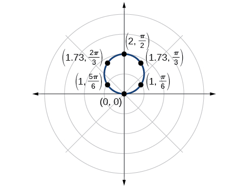
The point \(\left(2,\dfrac{\pi}{2}\right)\) will be the maximum value on the graph. Let’s plot a few more points to verify the graph of a circle. See Table \(\PageIndex{1}\) and Figure \(\PageIndex{4}\).

Table \(\PageIndex{1}\)

\(\theta\)	\(r=2 \sin \theta\)	\(r\)
\(0\)	\(r=2 \sin(0)=0\)	\(0\)
\(\dfrac{\pi}{6}\)	\(r=2 \sin\left(\dfrac{\pi}{6}\right)=1\)	\(1\)
\(\dfrac{\pi}{3}\)	\(r=2 \sin\left(\dfrac{\pi}{3}\right)≈1.73\)	\(1.73\)
\(\dfrac{pi}{2}\)	\(r=2 \sin\left(\dfrac{\pi}{2}\right)=2\)	\(2\)
\(\dfrac{2\pi}{3}\)	\(r=2 \sin\left(\dfrac{2\pi}{3}\right)≈1.73\)	\(1.73\)
\(\dfrac{5\pi}{6}\)	\(r=2 \sin\left(\dfrac{5\pi}{6}\right)=1\)	\(1\)
\(\pi\)	\(r=2 \sin(\pi)=0\)	\(0\)

Figure \(\PageIndex{4}\)

Investigating Circles

Now we have seen the equation of a circle in the polar coordinate system. In the last two examples, the same equation was used to illustrate the properties of symmetry and demonstrate how to find the zeros, maximum values, and plotted points that produced the graphs. However, the circle is only one of many shapes in the set of polar curves.

There are five classic polar curves: cardioids, limaҫons, lemniscates, rose curves, and Archimedes’ spirals. We will briefly touch on the polar formulas for the circle before moving on to the classic curves and their variations.

FORMULAS FOR THE EQUATION OF A CIRCLE

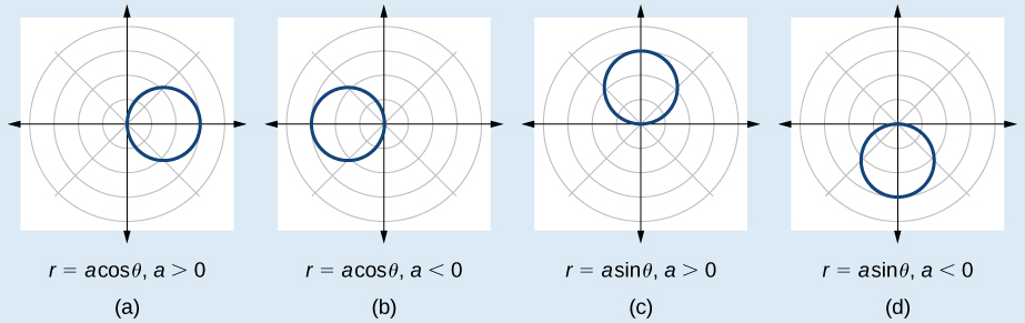
Some of the formulas that produce the graph of a circle in polar coordinates are given by \(r=a \cos \theta\) and \(r=a \sin \theta\), wherea a is the diameter of the circle or the distance from the pole to the farthest point on the circumference. The radius is \(\dfrac{|a|}{2}\), or one-half the diameter. For \(r=a \cos \theta\), the center is \(\left(\dfrac{a}{2},0\right)\). For \(r=a \sin \theta\), the center is \(\left(\dfrac{a}{2},\pi\right)\). Figure \(\PageIndex{5}\) shows the graphs of these four circles.

Figure \(\PageIndex{5}\)

Example \(\PageIndex{3}\): Sketching the Graph of a Polar Equation for a Circle

Sketch the graph of \(r=4 \cos \theta\).

Solution

First, testing the equation for symmetry, we find that the graph is symmetric about the polar axis. Next, we find the zeros and maximum \(| r |\) for \(r=4 \cos \theta\). First, set \(r=0\), and solve for \(\theta\). Thus, a zero occurs at \(\theta=\dfrac{\pi}{2}\pm k\pi\). A key point to plot is \(\left(0,\dfrac{\pi}{2}\right)\).

To find the maximum value of \(r\), note that the maximum value of the cosine function is \(1\) when \(\theta=0\pm 2k\pi\). Substitute \(\theta=0\) into the equation:

\[\begin{align*} r&= 4 \cos \theta\\ r&= 4 \cos(0)\\ r&= 4(1)\\ &= 4 \end{align*}\]

The maximum value of the equation is \(4\). A key point to plot is \((4, 0)\).

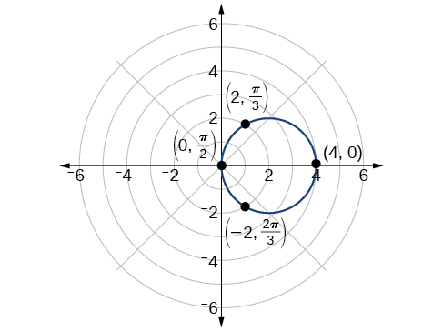
As \(r=4 \cos \theta\) is symmetric with respect to the polar axis, we only need to calculate \(r\)-values for \(θ\) over the interval \([0, \pi]\). Points in the upper quadrant can then be reflected to the lower quadrant. Make a table of values similar to Table \(\PageIndex{2}\). The graph is shown in Figure \(\PageIndex{6}\).

Table \(\PageIndex{2}\)

\(\theta\)	\(0\)	\(\dfrac{\pi}{6}\)	\(\dfrac{\pi}{4}\)	\(\dfrac{\pi}{3}\)	\(\dfrac{\pi}{2}\)	\(\dfrac{2\pi}{3}\)	\(\dfrac{3\pi}{4}\)	\(\dfrac{5\pi}{6}\)	\(\pi\)
\(r\)	\(4\)	\(3.46\)	\(2.83\)	\(2\)	\(0\)	\(−2\)	\(−2.83\)	\(−3.46\)	\(4\)

Figure \(\PageIndex{6}\)

Investigating Cardioids

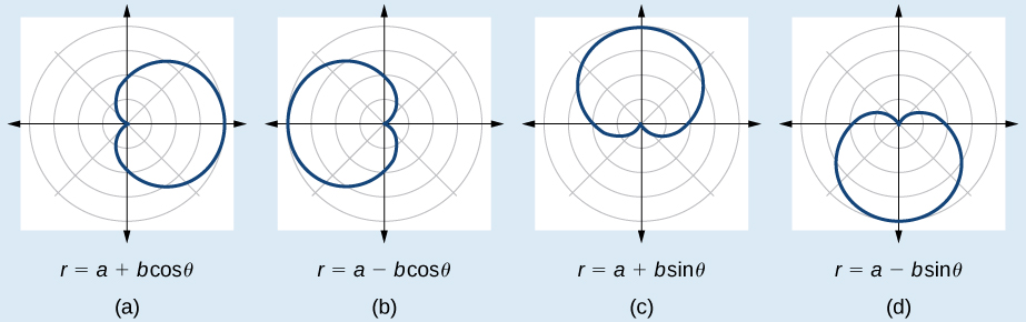
While translating from polar coordinates to Cartesian coordinates may seem simpler in some instances, graphing the classic curves is actually less complicated in the polar system. The next curve is called a cardioid, as it resembles a heart. This shape is often included with the family of curves called limaçons, but here we will discuss the cardioid on its own.

FORMULAS FOR A CARDIOID

The formulas that produce the graphs of a cardioid are given by \(r=a\pm b \cos \theta\) and \(r=a\pm b \sin \theta\) where \(a>0\), \(b>0\), and \(\dfrac{a}{b}=1\). The cardioid graph passes through the pole, as we can see in Figure \(\PageIndex{7}\).

Figure \(\PageIndex{7}\)

How to: Given the polar equation of a cardioid, sketch its graph

1. Check equation for the three types of symmetry.
2. Find the zeros. Set \(r=0\).
3. Find the maximum value of the equation according to the maximum value of the trigonometric expression.
4. Make a table of values for \(r\) and \(\theta\).
5. Plot the points and sketch the graph.

Example \(\PageIndex{4}\): Sketching the Graph of a Cardioid

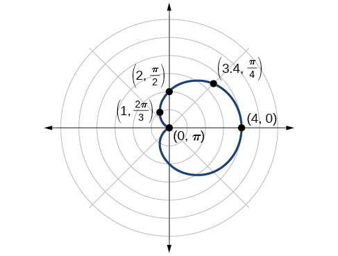
Sketch the graph of \(r=2+2 \cos \theta\).

Solution

First, testing the equation for symmetry, we find that the graph of this equation will be symmetric about the polar axis. Next, we find the zeros and maximums. Setting \(r=0\), we have \(\theta=\pi+2k\pi\). The zero of the equation is located at \((0,\pi)\). The graph passes through this point.

The maximum value of \(r=2+2 \cos \theta\) occurs when \(\cos \theta\) is a maximum, which is when \(\cos \theta=1\) or when \(\theta=0\). Substitute \(\theta=0\) into the equation, and solve for \(r\).

\[\begin{align*} r&= 2+2 \cos(0)\\ r&= 2+2(1)\\ &= 4 \end{align*}\]

The point \((4,0)\) is the maximum value on the graph.

We found that the polar equation is symmetric with respect to the polar axis, but as it extends to all four quadrants, we need to plot values over the interval \([0, \pi]\). The upper portion of the graph is then reflected over the polar axis. Next, we make a table of values, as in Table \(\PageIndex{3}\), and then we plot the points and draw the graph. See Figure \(\PageIndex{8}\).

Table \(\PageIndex{3}\)

θ	0	\(\dfrac{π}{4}\)	\(\dfrac{π}{2}\)	\(\dfrac{2π}{3}\)	\(π\)
r	4	3.41	2	1	0

Figure \(\PageIndex{8}\)

Investigating the Archimedes’ Spiral

The final polar equation we will discuss is the Archimedes’ spiral, named for its discoverer, the Greek mathematician Archimedes (c. 287 BCE - c. 212 BCE), who is credited with numerous discoveries in the fields of geometry and mechanics.

ARCHIMEDES’ SPIRAL

The formula that generates the graph of the Archimedes’ spiral is given by \(r=\theta\) for \(\theta≥0\). As \(\theta\) increases, \(r\) increases at a constant rate in an ever-widening, never-ending, spiraling path. See Figure \(\PageIndex{21}\).

Figure \(\PageIndex{21}\)

How to: Given an Archimedes’ spiral over \([ 0,2\pi ]\),sketch the graph

1. Make a table of values for \(r\) and \(\theta\) over the given domain.
2. Plot the points and sketch the graph.

Example \(\PageIndex{10}\): Sketching the Graph of an Archimedes’ Spiral

Sketch the graph of \(r=\theta\) over \([0,2\pi]\).

Solution

As \(r\) is equal to \(\theta\), the plot of the Archimedes’ spiral begins at the pole at the point \((0, 0)\). While the graph hints of symmetry, there is no formal symmetry with regard to passing the symmetry tests. Further, there is no maximum value, unless the domain is restricted.

Create a table such as Table \(\PageIndex{9}\).

Table \(\PageIndex{9}\)

\(\theta\)	\(\dfrac{\pi}{4}\)	\(\dfrac{\pi}{2}\)	\(\pi\)	\(\dfrac{3\pi}{2}\)	\(\dfrac{7\pi}{4}\)	\(2\pi\)
\(r\)	\(0.785\)	\(1.57\)	\(3.14\)	\(4.71\)	\(5.50\)	\(6.28\)

Notice that the r-values are just the decimal form of the angle measured in radians. We can see them on a graph in Figure \(\PageIndex{22}\).

Figure \(\PageIndex{22}\): Archimedes’ spiral

Analysis

The domain of this polar curve is \([ 0,2\pi ]\). In general, however, the domain of this function is \((−\infty,\infty)\). Graphing the equation of the Archimedes’ spiral is rather simple, although the image makes it seem like it would be complex.