6.3: Fractals

Last updated
Save as PDF

Page ID: 74342

Leah Griffith, Veronica Holbrook, Johnny Johnson & Nancy Garcia
Rio Hondo College

$ \newcommand{\vecs}[1]{\overset { \scriptstyle \rightharpoonup} {\mathbf{#1}} } $

$ \newcommand{\vecd}[1]{\overset{-\!-\!\rightharpoonup}{\vphantom{a}\smash {#1}}} $

$ \newcommand{\id}{\mathrm{id}}$ $ \newcommand{\Span}{\mathrm{span}}$

( \newcommand{\kernel}{\mathrm{null}\,}\) $ \newcommand{\range}{\mathrm{range}\,}$

$ \newcommand{\RealPart}{\mathrm{Re}}$ $ \newcommand{\ImaginaryPart}{\mathrm{Im}}$

$ \newcommand{\Argument}{\mathrm{Arg}}$ $ \newcommand{\norm}[1]{\| #1 \|}$

$ \newcommand{\inner}[2]{\langle #1, #2 \rangle}$

$ \newcommand{\Span}{\mathrm{span}}$

$ \newcommand{\id}{\mathrm{id}}$

$ \newcommand{\Span}{\mathrm{span}}$

$ \newcommand{\kernel}{\mathrm{null}\,}$

$ \newcommand{\range}{\mathrm{range}\,}$

$ \newcommand{\RealPart}{\mathrm{Re}}$

$ \newcommand{\ImaginaryPart}{\mathrm{Im}}$

$ \newcommand{\Argument}{\mathrm{Arg}}$

$ \newcommand{\norm}[1]{\| #1 \|}$

$ \newcommand{\inner}[2]{\langle #1, #2 \rangle}$

$ \newcommand{\Span}{\mathrm{span}}$ $ \newcommand{\AA}{\unicode[.8,0]{x212B}}$

$ \newcommand{\vectorA}[1]{\vec{#1}} % arrow$

$ \newcommand{\vectorAt}[1]{\vec{\text{#1}}} % arrow$

$ \newcommand{\vectorB}[1]{\overset { \scriptstyle \rightharpoonup} {\mathbf{#1}} } $

$ \newcommand{\vectorC}[1]{\textbf{#1}} $

$ \newcommand{\vectorD}[1]{\overrightarrow{#1}} $

$ \newcommand{\vectorDt}[1]{\overrightarrow{\text{#1}}} $

$ \newcommand{\vectE}[1]{\overset{-\!-\!\rightharpoonup}{\vphantom{a}\smash{\mathbf {#1}}}} $

$ \newcommand{\vecs}[1]{\overset { \scriptstyle \rightharpoonup} {\mathbf{#1}} } $

$ \newcommand{\vecd}[1]{\overset{-\!-\!\rightharpoonup}{\vphantom{a}\smash {#1}}} $

$\newcommand{\avec}{\mathbf a}$ $\newcommand{\bvec}{\mathbf b}$ $\newcommand{\cvec}{\mathbf c}$ $\newcommand{\dvec}{\mathbf d}$ $\newcommand{\dtil}{\widetilde{\mathbf d}}$ $\newcommand{\evec}{\mathbf e}$ $\newcommand{\fvec}{\mathbf f}$ $\newcommand{\nvec}{\mathbf n}$ $\newcommand{\pvec}{\mathbf p}$ $\newcommand{\qvec}{\mathbf q}$ $\newcommand{\svec}{\mathbf s}$ $\newcommand{\tvec}{\mathbf t}$ $\newcommand{\uvec}{\mathbf u}$ $\newcommand{\vvec}{\mathbf v}$ $\newcommand{\wvec}{\mathbf w}$ $\newcommand{\xvec}{\mathbf x}$ $\newcommand{\yvec}{\mathbf y}$ $\newcommand{\zvec}{\mathbf z}$ $\newcommand{\rvec}{\mathbf r}$ $\newcommand{\mvec}{\mathbf m}$ $\newcommand{\zerovec}{\mathbf 0}$ $\newcommand{\onevec}{\mathbf 1}$ $\newcommand{\real}{\mathbb R}$ $\newcommand{\twovec}[2]{\left[\begin{array}{r}#1 \\ #2 \end{array}\right]}$ $\newcommand{\ctwovec}[2]{\left[\begin{array}{c}#1 \\ #2 \end{array}\right]}$ $\newcommand{\threevec}[3]{\left[\begin{array}{r}#1 \\ #2 \\ #3 \end{array}\right]}$ $\newcommand{\cthreevec}[3]{\left[\begin{array}{c}#1 \\ #2 \\ #3 \end{array}\right]}$ $\newcommand{\fourvec}[4]{\left[\begin{array}{r}#1 \\ #2 \\ #3 \\ #4 \end{array}\right]}$ $\newcommand{\cfourvec}[4]{\left[\begin{array}{c}#1 \\ #2 \\ #3 \\ #4 \end{array}\right]}$ $\newcommand{\fivevec}[5]{\left[\begin{array}{r}#1 \\ #2 \\ #3 \\ #4 \\ #5 \\ \end{array}\right]}$ $\newcommand{\cfivevec}[5]{\left[\begin{array}{c}#1 \\ #2 \\ #3 \\ #4 \\ #5 \\ \end{array}\right]}$ $\newcommand{\mattwo}[4]{\left[\begin{array}{rr}#1 \amp #2 \\ #3 \amp #4 \\ \end{array}\right]}$ $\newcommand{\laspan}[1]{\text{Span}\{#1\}}$ $\newcommand{\bcal}{\cal B}$ $\newcommand{\ccal}{\cal C}$ $\newcommand{\scal}{\cal S}$ $\newcommand{\wcal}{\cal W}$ $\newcommand{\ecal}{\cal E}$ $\newcommand{\coords}[2]{\left\{#1\right\}_{#2}}$ $\newcommand{\gray}[1]{\color{gray}{#1}}$ $\newcommand{\lgray}[1]{\color{lightgray}{#1}}$ $\newcommand{\rank}{\operatorname{rank}}$ $\newcommand{\row}{\text{Row}}$ $\newcommand{\col}{\text{Col}}$ $\renewcommand{\row}{\text{Row}}$ $\newcommand{\nul}{\text{Nul}}$ $\newcommand{\var}{\text{Var}}$ $\newcommand{\corr}{\text{corr}}$ $\newcommand{\len}[1]{\left|#1\right|}$ $\newcommand{\bbar}{\overline{\bvec}}$ $\newcommand{\bhat}{\widehat{\bvec}}$ $\newcommand{\bperp}{\bvec^\perp}$ $\newcommand{\xhat}{\widehat{\xvec}}$ $\newcommand{\vhat}{\widehat{\vvec}}$ $\newcommand{\uhat}{\widehat{\uvec}}$ $\newcommand{\what}{\widehat{\wvec}}$ $\newcommand{\Sighat}{\widehat{\Sigma}}$ $\newcommand{\lt}{<}$ $\newcommand{\gt}{>}$ $\newcommand{\amp}{&}$ $\definecolor{fillinmathshade}{gray}{0.9}$

Fractals are mathematical sets, usually obtained through recursion, that exhibit interesting dimensional properties. We’ll explore what that sentence means through the rest of the chapter. For now, we can begin with the idea of self-similarity, a characteristic of most fractals.

Definition: Self-Similarity

A shape is self-similar when it looks essentially the same from a distance as it does closer up.

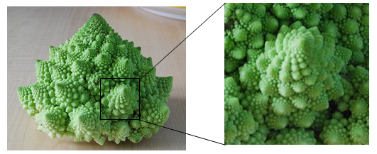
Self-similarity can often be found in nature. In the Romanesco broccoli pictured below[1], if we zoom in on part of the image, the piece remaining looks similar to the whole.

$A picture of Romanesco Broccoli with an inset that zooms in to see that the overall shape of the broccoli repeats in the inner part of the broccoli.$

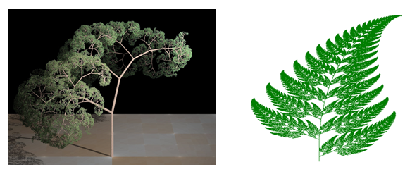
Likewise, in the fern frond below[2], one piece of the frond looks similar to the whole.

$A fern frond with many leaves. One leaf is zoomed in on to see that it repeats the pattern of the larger frond.$

Similarly, if we zoom in on the coastline of Portugal[3], each zoom reveals previously hidden detail, and the coastline, while not identical to the view from further way, does exhibit similar characteristics.

$The coastline of Portugal zoomed in twice to see the similar patterns in the coastline at the three different levels of focus.$

This self-similar behavior can be replicated through recursion: repeating a process over and over.

Example 1

Suppose that we start with a filled-in triangle. We connect the midpoints of each side and remove the middle triangle. We then repeat this process.

$The initial step of the pattern is a solid equilateral triangle. The second step cuts out one triangle from the center whose vertices connect to the midpoint of each of the original triangles sides. This forms three smaller solid triangles within the original triangle. Step 3 repeat the cutout process in the three newly formed solid triangles, forming three smaller solid triangles within the previous step's solid triangel. The forth step repeats the cutout process with the nine newly formed solid triangles.$

If we repeat this process, the shape that emerges is called the Sierpinski gasket. Notice that it exhibits self-similarity – any piece of the gasket will look identical to the whole. In fact, we can say that the Sierpinski gasket contains three copies of itself, each half as tall and wide as the original. Of course, each of those copies also contains three copies of itself.

$The larger triangle with many iterations of cutouts is shown with one sectioned zoomed in to that shows the pattern continues at every level of focus.$

We can construct other fractals using a similar approach. To formalize this a bit, we’re going to introduce the idea of initiators and generators.

Definition: Initiators and Generators

An initiator is a starting shape
A generator is an arranged collection of scaled copies of the initiator

To generate fractals from initiators and generators, we follow a simple rule:

Fractal Generation Rule

At each step, replace every copy of the initiator with a scaled copy of the generator, rotating as necessary

This process is easiest to understand through example.

Example 2

Use the initiator and generator shown to create the iterated fractal.

$The initiator is a straight line segment. The generator is the same length but cut into thirds, with the middle third replaced by a triangular peak with left and right sides of equal length and no base.$

Solution

This tells us to, at each step, replace each line segment with the spiked shape shown in the generator. Notice that the generator itself is made up of 4 copies of the initiator. In step 1, the single line segment in the initiator is replaced with the generator. For step 2, each of the four line segments of step 1 is replaced with a scaled copy of the generator:

$This shows the first three steps of replacing a line segment with the spiked generator. Each reduced size line segment that is formed from being replaced by the generator is also replaced with a smaller version of the generator.$

This process is repeated to form Step 3. Again, each line segment is replaced with a scaled copy of the generator.

$The above process continues with replacing line segments with the peaked generator.$

Notice that since Step 0 only had 1 line segment, Step 1 only required one copy of Step 0.

Since Step 1 had 4 line segments, Step 2 required 4 copies of the generator.

Step 2 then had 16 line segments, so Step 3 required 16 copies of the generator.

Step 4, then, would require $16 \times 4 = 64$ copies of the generator.

The shape resulting from iterating this process is called the Koch curve, named for Helge von Koch who first explored it in 1904.

$The formal name of the process described above is the Koch curve.$

Notice that the Sierpinski gasket can also be described using the initiator-generator approach

$The same image from the first fractal formed above using a solid triangle in the first step and cuting out a triangle whose vertices are at the midpoint of each side.$

Example 3

Use the initiator and generator below, however only iterate on the “branches.” Sketch several steps of the iteration.

$The initiator is a vertical line segment. The generator attaches two the line segments that are half the length of the original segment to the top of the segment so that it forms a V$

Solution

We begin by replacing the initiator with the generator. We then replace each “branch” of Step 1 with a scaled copy of the generator to create Step 2.

$After replacing the original line segment with the generator, the process is repeated to add two more line segments, half the size of the previous segment at the end to form a V. This is done for both of the new segments so that there are now four new line segments on the previous two that were created.$

We can repeat this process to create later steps. Repeating this process can create intricate tree shapes[1].

$This shows three more steps of attaching half size line segments as a V at the top of the previous line segment, which eventually forms a shape that resembles a tree with no leaves.$

Try it Now 1

Use the initiator and generator shown to produce the next two stages

$The initiator is a solid pentagon. The generator repaces the original pentagon, with 5 smaller pentagons, with their top vertex at each of the vertices of the original pentagon.$

Answer: $Step two shows the 5 smaller pentagons each being replaced with 5 pentagons that are even smaller so they fit within the space of the original 5 pentagons. The fourth step repeats that process for each of the pentagons generated in step 3.$

Using iteration processes like those above can create a variety of beautiful images evocative of nature[2][3].

$The first image shows a plant branch that has leaves that follow a pattern that resembles the fractal process. A second image shows a fern frond.$

More natural shapes can be created by adding in randomness to the steps.

Example 4

Create a variation on the Sierpinski gasket by randomly skewing the corner points each time an iteration is made.

Solution

Suppose we start with the triangle below. We begin, as before, by removing the middle triangle. We then add in some randomness.

$The initiator is an obtuse triangle. The generator connects the midpoint of each side to cutout an internal triangle. The next step shows the figure with added randomness meaning the inner triangle is rotated and the connecting vertices of the outer triangle stay connected so that the outer triangle is distorted.$

We then repeat this process.

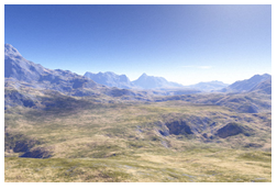
$This image begins with the randomized triangle from the previous image. It cuts out a central triangle from the three newly generated solid triangles connecting the midpoints. The inner cutouts are rotated to add more randomness to the figure. A third step repeats that process.$

Continuing this process can create mountain-like structures.

The landscape below was created using fractals, then colored and textured.

$An image of a computer generated mountain range that was done using fractals and randomness$

[1] http://www.flickr.com/photos/visualarts/5436068969/

[2] en.Wikipedia.org/wiki/File:Fr...e_b_-_2%29.jpg

[3] en.Wikipedia.org/wiki/File:Ba...-_4_states.PNG

[4] en.Wikipedia.org/wiki/File:Fr...lLandscape.jpg

[1] en.Wikipedia.org/wiki/File:Ca...ractal_AVM.JPG

[2] http://www.flickr.com/photos/cjewel/3261398909/

[3] Openstreetmap.org, CC-BY-SA

Search

Text Color

Text Size

Margin Size

Font Type