6.1: Polar Coordinates

Last updated
Save as PDF

Page ID: 61269

$ \newcommand{\vecs}[1]{\overset { \scriptstyle \rightharpoonup} {\mathbf{#1}} } $

$ \newcommand{\vecd}[1]{\overset{-\!-\!\rightharpoonup}{\vphantom{a}\smash {#1}}} $

$ \newcommand{\id}{\mathrm{id}}$ $ \newcommand{\Span}{\mathrm{span}}$

( \newcommand{\kernel}{\mathrm{null}\,}\) $ \newcommand{\range}{\mathrm{range}\,}$

$ \newcommand{\RealPart}{\mathrm{Re}}$ $ \newcommand{\ImaginaryPart}{\mathrm{Im}}$

$ \newcommand{\Argument}{\mathrm{Arg}}$ $ \newcommand{\norm}[1]{\| #1 \|}$

$ \newcommand{\inner}[2]{\langle #1, #2 \rangle}$

$ \newcommand{\Span}{\mathrm{span}}$

$ \newcommand{\id}{\mathrm{id}}$

$ \newcommand{\Span}{\mathrm{span}}$

$ \newcommand{\kernel}{\mathrm{null}\,}$

$ \newcommand{\range}{\mathrm{range}\,}$

$ \newcommand{\RealPart}{\mathrm{Re}}$

$ \newcommand{\ImaginaryPart}{\mathrm{Im}}$

$ \newcommand{\Argument}{\mathrm{Arg}}$

$ \newcommand{\norm}[1]{\| #1 \|}$

$ \newcommand{\inner}[2]{\langle #1, #2 \rangle}$

$ \newcommand{\Span}{\mathrm{span}}$ $ \newcommand{\AA}{\unicode[.8,0]{x212B}}$

$ \newcommand{\vectorA}[1]{\vec{#1}} % arrow$

$ \newcommand{\vectorAt}[1]{\vec{\text{#1}}} % arrow$

$ \newcommand{\vectorB}[1]{\overset { \scriptstyle \rightharpoonup} {\mathbf{#1}} } $

$ \newcommand{\vectorC}[1]{\textbf{#1}} $

$ \newcommand{\vectorD}[1]{\overrightarrow{#1}} $

$ \newcommand{\vectorDt}[1]{\overrightarrow{\text{#1}}} $

$ \newcommand{\vectE}[1]{\overset{-\!-\!\rightharpoonup}{\vphantom{a}\smash{\mathbf {#1}}}} $

$ \newcommand{\vecs}[1]{\overset { \scriptstyle \rightharpoonup} {\mathbf{#1}} } $

$ \newcommand{\vecd}[1]{\overset{-\!-\!\rightharpoonup}{\vphantom{a}\smash {#1}}} $

$\newcommand{\avec}{\mathbf a}$ $\newcommand{\bvec}{\mathbf b}$ $\newcommand{\cvec}{\mathbf c}$ $\newcommand{\dvec}{\mathbf d}$ $\newcommand{\dtil}{\widetilde{\mathbf d}}$ $\newcommand{\evec}{\mathbf e}$ $\newcommand{\fvec}{\mathbf f}$ $\newcommand{\nvec}{\mathbf n}$ $\newcommand{\pvec}{\mathbf p}$ $\newcommand{\qvec}{\mathbf q}$ $\newcommand{\svec}{\mathbf s}$ $\newcommand{\tvec}{\mathbf t}$ $\newcommand{\uvec}{\mathbf u}$ $\newcommand{\vvec}{\mathbf v}$ $\newcommand{\wvec}{\mathbf w}$ $\newcommand{\xvec}{\mathbf x}$ $\newcommand{\yvec}{\mathbf y}$ $\newcommand{\zvec}{\mathbf z}$ $\newcommand{\rvec}{\mathbf r}$ $\newcommand{\mvec}{\mathbf m}$ $\newcommand{\zerovec}{\mathbf 0}$ $\newcommand{\onevec}{\mathbf 1}$ $\newcommand{\real}{\mathbb R}$ $\newcommand{\twovec}[2]{\left[\begin{array}{r}#1 \\ #2 \end{array}\right]}$ $\newcommand{\ctwovec}[2]{\left[\begin{array}{c}#1 \\ #2 \end{array}\right]}$ $\newcommand{\threevec}[3]{\left[\begin{array}{r}#1 \\ #2 \\ #3 \end{array}\right]}$ $\newcommand{\cthreevec}[3]{\left[\begin{array}{c}#1 \\ #2 \\ #3 \end{array}\right]}$ $\newcommand{\fourvec}[4]{\left[\begin{array}{r}#1 \\ #2 \\ #3 \\ #4 \end{array}\right]}$ $\newcommand{\cfourvec}[4]{\left[\begin{array}{c}#1 \\ #2 \\ #3 \\ #4 \end{array}\right]}$ $\newcommand{\fivevec}[5]{\left[\begin{array}{r}#1 \\ #2 \\ #3 \\ #4 \\ #5 \\ \end{array}\right]}$ $\newcommand{\cfivevec}[5]{\left[\begin{array}{c}#1 \\ #2 \\ #3 \\ #4 \\ #5 \\ \end{array}\right]}$ $\newcommand{\mattwo}[4]{\left[\begin{array}{rr}#1 \amp #2 \\ #3 \amp #4 \\ \end{array}\right]}$ $\newcommand{\laspan}[1]{\text{Span}\{#1\}}$ $\newcommand{\bcal}{\cal B}$ $\newcommand{\ccal}{\cal C}$ $\newcommand{\scal}{\cal S}$ $\newcommand{\wcal}{\cal W}$ $\newcommand{\ecal}{\cal E}$ $\newcommand{\coords}[2]{\left\{#1\right\}_{#2}}$ $\newcommand{\gray}[1]{\color{gray}{#1}}$ $\newcommand{\lgray}[1]{\color{lightgray}{#1}}$ $\newcommand{\rank}{\operatorname{rank}}$ $\newcommand{\row}{\text{Row}}$ $\newcommand{\col}{\text{Col}}$ $\renewcommand{\row}{\text{Row}}$ $\newcommand{\nul}{\text{Nul}}$ $\newcommand{\var}{\text{Var}}$ $\newcommand{\corr}{\text{corr}}$ $\newcommand{\len}[1]{\left|#1\right|}$ $\newcommand{\bbar}{\overline{\bvec}}$ $\newcommand{\bhat}{\widehat{\bvec}}$ $\newcommand{\bperp}{\bvec^\perp}$ $\newcommand{\xhat}{\widehat{\xvec}}$ $\newcommand{\vhat}{\widehat{\vvec}}$ $\newcommand{\uhat}{\widehat{\uvec}}$ $\newcommand{\what}{\widehat{\wvec}}$ $\newcommand{\Sighat}{\widehat{\Sigma}}$ $\newcommand{\lt}{<}$ $\newcommand{\gt}{>}$ $\newcommand{\amp}{&}$ $\definecolor{fillinmathshade}{gray}{0.9}$

Learning Objectives

Distinguish between and understand the difference between a rectangular coordinate system and a polar coordinate system.
Plot points with polar coordinates on a polar plane.

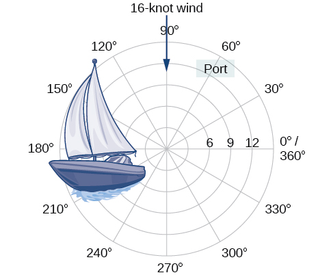
Over $12$ kilometers from port, a sailboat encounters rough weather and is blown off course by a $16$-knot wind (see Figure $\PageIndex{1}$). How can the sailor indicate his location to the Coast Guard? In this section, we will investigate a method of representing location that is different from a standard coordinate grid.

An illustration of a boat on the polar grid. — Figure $\PageIndex{1}$

Plotting Points Using Polar Coordinates

When we think about plotting points in the plane, we usually think of rectangular coordinates $(x,y)$ in the Cartesian coordinate plane. However, there are other ways of writing a coordinate pair and other types of grid systems. In this section, we introduce to polar coordinates, which are points labeled $(r,\theta)$ and plotted on a polar grid. The polar grid is represented as a series of concentric circles radiating out from the pole, or the origin of the coordinate plane.

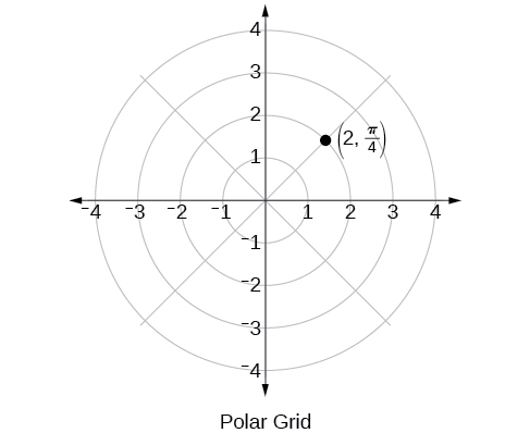
The polar grid is scaled as the unit circle with the positive $x$-axis now viewed as the polar axis and the origin as the pole. The first coordinate $r$ is the radius or length of the directed line segment from the pole. The angle $\theta$, measured in radians, indicates the direction of $r$. We move counterclockwise from the polar axis by an angle of $\theta$,and measure a directed line segment the length of $r$ in the direction of $\theta$. Even though we measure $\theta$ first and then $r$, the polar point is written with the $r$-coordinate first. For example, to plot the point $\left(2,\dfrac{\pi}{4}\right)$, we would move $\dfrac{\pi}{4}$ units in the counterclockwise direction and then a length of $2$ from the pole. This point is plotted on the grid in Figure $\PageIndex{2}$.

Polar grid with point (2, pi/4) plotted. — Figure $\PageIndex{2}$

Example $\PageIndex{1}$: Plotting a Point on the Polar Grid

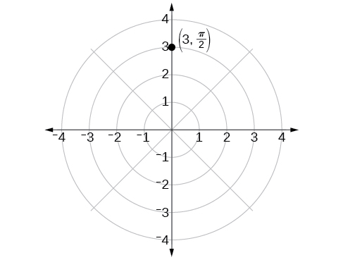
Plot the point $\left(3,\dfrac{\pi}{2}\right)$ on the polar grid.

Solution

The angle $\dfrac{\pi}{2}$ is found by sweeping in a counterclockwise direction $90°$ from the polar axis. The point is located at a length of $3$ units from the pole in the $\dfrac{\pi}{2}$ direction, as shown in Figure $\PageIndex{3}$.

Polar grid with point (3, pi/2) plotted. — Figure $\PageIndex{3}$

Exercise $\PageIndex{1}$

Plot the point $\left(2, \dfrac{\pi}{3}\right)$ in the polar grid.

Answer: $Polar grid with point (2, pi/3) plotted.$
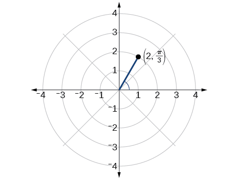
Figure $\PageIndex{4}$

Example $\PageIndex{2}$: Plotting a Point in the Polar Coordinate System with a Negative Component

Plot the point $\left(−2, \dfrac{\pi}{6}\right)$ on the polar grid.

Solution

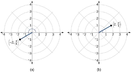
We know that $\dfrac{\pi}{6}$ is located in the first quadrant. However, $r=−2$. We can approach plotting a point with a negative $r$ in two ways:

Plot the point $\left(2,\dfrac{\pi}{6}\right)$ by moving $\dfrac{\pi}{6}$ in the counterclockwise direction and extending a directed line segment $2$ units into the first quadrant. Then retrace the directed line segment back through the pole, and continue $2$ units into the third quadrant;
Move $\dfrac{\pi}{6}$ in the counterclockwise direction, and draw the directed line segment from the pole $2$ units in the negative direction, into the third quadrant.

See Figure $\PageIndex{5a}$. Compare this to the graph of the polar coordinate $\left(2,\dfrac{\pi}{6}\right)$ shown in Figure $\PageIndex{5b}$.

Two polar grids. Points (2, pi/6) and (-2, pi/6) are plotted. They are reflections across the origin in Q1 and Q3. — Figure $\PageIndex{5}$

Exercise $\PageIndex{2}$

Plot the points $\left(3,−\dfrac{\pi}{6}\right)$ and $\left(2,\dfrac{9\pi}{4}\right)$ on the same polar grid.

Answer: $Points (2, 9pi/4) and (3, -pi/6) are plotted in the polar grid.$
Figure $\PageIndex{6}$

Converting from Polar Coordinates to Rectangular Coordinates

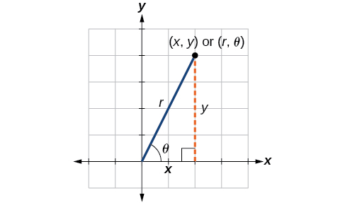
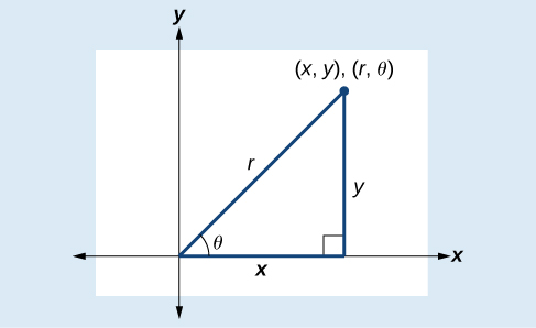
When given a set of polar coordinates, we may need to convert them to rectangular coordinates. To do so, we can recall the relationships that exist among the variables $x$, $y$, $r$, and $\theta$.

$\cos \theta=\dfrac{x}{r}\rightarrow x=r \cos \theta$

$\sin \theta=\dfrac{y}{r}\rightarrow y=r \sin \theta$

Dropping a perpendicular from the point in the plane to the x-axis forms a right triangle, as illustrated in Figure $\PageIndex{7}$. An easy way to remember the equations above is to think of $\cos \theta$ as the adjacent side over the hypotenuse and $\sin \theta$ as the opposite side over the hypotenuse.

Comparison between polar coordinates and rectangular coordinates. There is a right triangle plotted on the x,y axis. The sides are a horizontal line on the x-axis of length x, a vertical line extending from thex-axis to some point in quadrant 1, and a hypotenuse r extending from the origin to that same point in quadrant 1. The vertices are at the origin (0,0), some point along the x-axis at (x,0), and that point in quadrant 1. This last point is (x,y) or (r, theta), depending which system of coordinates you use. — Figure $\PageIndex{7}$

CONVERTING FROM POLAR COORDINATES TO RECTANGULAR COORDINATES

To convert polar coordinates $(r, \theta)$ to rectangular coordinates $(x, y)$, let

\[\cos \theta=\dfrac{x}{r}\rightarrow x=r \cos \theta\]

\[\sin \theta=\dfrac{y}{r}\rightarrow y=r \sin \theta\]

How to: Given polar coordinates, convert to rectangular coordinates.

Given the polar coordinate $(r,\theta)$, write $x=r \cos \theta$ and $y=r \sin \theta$.
Evaluate $\cos \theta$ and $\sin \theta$.
Multiply $\cos \theta$ by $r$ to find the $x$-coordinate of the rectangular form.
Multiply $\sin \theta$ by $r$ to find the $y$-coordinate of the rectangular form.

Example $\PageIndex{3A}$: Writing Polar Coordinates as Rectangular Coordinates

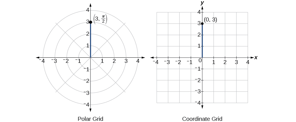
Write the polar coordinates $\left(3,\dfrac{\pi}{2}\right)$ as rectangular coordinates.

Solution

Use the equivalent relationships.

\[\begin{align*} x&= r \cos \theta\\ x&= 3 \cos \dfrac{\pi}{2}\\ &= 0\\ y&= r \sin \theta\\ y&= 3 \sin \dfrac{\pi}{2}\\ &= 3 \end{align*}\]

The rectangular coordinates are $(0,3)$. See Figure $\PageIndex{8}$.

Illustration of (3, pi/2) in polar coordinates and (0,3) in rectangular coordinates - they are the same point! — Figure $\PageIndex{8}$

Example $\PageIndex{3B}$: Writing Polar Coordinates as Rectangular Coordinates

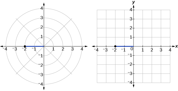
Write the polar coordinates $(−2,0)$ as rectangular coordinates.

Solution

See Figure $\PageIndex{9}$. Writing the polar coordinates as rectangular, we have

\[\begin{align*} x&= r \cos \theta\\ x&= -2 \cos(0)\\ &= -2\\ y&= r \sin \theta\\ y&= -2 \sin(0)\\ &= 0 \end{align*}\]

The rectangular coordinates are also $(−2,0)$.

Illustration of (-2, 0) in polar coordinates and (-2,0) in rectangular coordinates - they are the same point! — Figure $\PageIndex{9}$

Exercise $\PageIndex{3}$

Write the polar coordinates $\left(−1,\dfrac{2\pi}{3}\right)$ as rectangular coordinates.

Answer: $(x,y)=\left(\dfrac{1}{2},−\dfrac{\sqrt{3}}{2}\right)$

Converting from Rectangular Coordinates to Polar Coordinates

To convert rectangular coordinates to polar coordinates, we will use two other familiar relationships. With this conversion, however, we need to be aware that a set of rectangular coordinates will yield more than one polar point.

CONVERTING FROM RECTANGULAR COORDINATES TO POLAR COORDINATES

Converting from rectangular coordinates to polar coordinates requires the use of one or more of the relationships illustrated in Figure $\PageIndex{10}$.

$\cos \theta=\dfrac{x}{r}$ or $x=r \cos \theta$

$\sin \theta=\dfrac{y}{r}$ or $y=r \sin \theta$

$r^2=x^2+y^2$

$\tan \theta=\dfrac{y}{x}$

Example $\PageIndex{4}$: Writing Rectangular Coordinates as Polar Coordinates

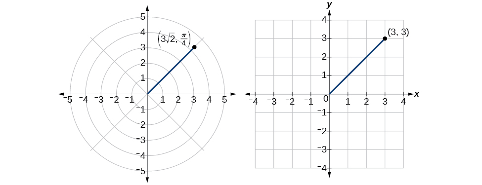
Convert the rectangular coordinates $(3,3)$ to polar coordinates.

Solution

We see that the original point $(3,3)$ is in the first quadrant. To find $\theta$, use the formula $\tan \theta=\dfrac{y}{x}$. This gives

\[\begin{align*} \tan \theta&= \dfrac{3}{3}\\ \tan \theta&= 1\\ {\tan}^{-1}(1)&= \dfrac{\pi}{4} \end{align*}\]

To find $r$, we substitute the values for $x$ and $y$ into the formula $r=\sqrt{x^2+y^2}$. We know that $r$ must be positive, as $\dfrac{\pi}{4}$ is in the first quadrant. Thus

\[\begin{align*} r&= \sqrt{3^2+3^2}\\ r&= \sqrt{9+9}\\ r&= \sqrt{18}\\ &= 3\sqrt{2} \end{align*}\]

So, $r=3\sqrt{2}$ and $\theta=\dfrac{\pi}{4}$, giving us the polar point $(3\sqrt{2},\dfrac{\pi}{4})$. See Figure $\PageIndex{11}$.

Illustration of (3rad2, pi/4) in polar coordinates and (3,3) in rectangular coordinates - they are the same point! — Figure $\PageIndex{11}$

Analysis

There are other sets of polar coordinates that will be the same as our first solution. For example, the points $\left(−3\sqrt{2}, \dfrac{5\pi}{4}\right)$ and $\left(3\sqrt{2},−\dfrac{7\pi}{4}\right)$ will coincide with the original solution of $\left(3\sqrt{2}, \dfrac{\pi}{4}\right)$. The point $\left(−3\sqrt{2}, \dfrac{5\pi}{4}\right)$ indicates a move further counterclockwise by $\pi$, which is directly opposite $\dfrac{\pi}{4}$. The radius is expressed as $−3\sqrt{2}$. However, the angle $\dfrac{5\pi}{4}$ is located in the third quadrant and, as $r$ is negative, we extend the directed line segment in the opposite direction, into the first quadrant. This is the same point as $\left(3\sqrt{2}, \dfrac{\pi}{4}\right)$. The point $\left(3\sqrt{2}, −\dfrac{7\pi}{4}\right)$ is a move further clockwise by $−\dfrac{7\pi}{4}$, from $\dfrac{\pi}{4}$. The radius, $3\sqrt{2}$, is the same.

Extra Practice

Plot the point with polar coordinates $\left(3, \frac{\pi}{6}\right)$.
Plot the point with polar coordinates $\left(5,-\frac{2 \pi}{3}\right)$
Convert $\left(6,-\frac{3 \pi}{4}\right)$ to rectangular coordinates.
Convert $\left(-2, \frac{3 \pi}{2}\right)$ to rectangular coordinates.
Convert (7,-2) to polar coordinates.
Convert (-9,-4) to polar coordinates.

Key Equations

Conversion formulas

$\cos \theta=\dfrac{x}{r} \rightarrow x=r \cos\theta$

$\sin \theta=\dfrac{y}{r} \rightarrow y=r \sin \theta$

$r^2=x^2+y^2$

$\tan \theta=\dfrac{y}{x}$

Key Concepts

The polar grid is represented as a series of concentric circles radiating out from the pole, or origin.
To plot a point in the form $(r,\theta)$, $\theta>0$, move in a counterclockwise direction from the polar axis by an angle of $\theta$, and then extend a directed line segment from the pole the length of $r$ in the direction of $\theta$. If $\theta$ is negative, move in a clockwise direction, and extend a directed line segment the length of $r$ in the direction of $\theta$. See Example $\PageIndex{1}$.
If $r$ is negative, extend the directed line segment in the opposite direction of $\theta$. See Example $\PageIndex{2}$.
To convert from polar coordinates to rectangular coordinates, use the formulas $x=r \cos \theta$ and $y=r \sin \theta$. See Example $\PageIndex{3}$ and Example $\PageIndex{4}$.
To convert from rectangular coordinates to polar coordinates, use one or more of the formulas: $\cos \theta=\dfrac{x}{r}$, $\sin \theta=\dfrac{y}{r}$, $\tan \theta=\dfrac{y}{x}$, and $r=\sqrt{x^2+y^2}$. See Example $\PageIndex{5}$.

Contributors and Attributions

Jay Abramson (Arizona State University) with contributing authors. Textbook content produced by OpenStax College is licensed under a Creative Commons Attribution License 4.0 license. Download for free at https://openstax.org/details/books/precalculus.

Search

Text Color

Text Size

Margin Size

Font Type