
4.4 Inverse Functions
- Page ID
- 153662

\( \newcommand{\vecs}[1]{\overset { \scriptstyle \rightharpoonup} {\mathbf{#1}} } \)
\( \newcommand{\vecd}[1]{\overset{-\!-\!\rightharpoonup}{\vphantom{a}\smash {#1}}} \)
\( \newcommand{\dsum}{\displaystyle\sum\limits} \)
\( \newcommand{\dint}{\displaystyle\int\limits} \)
\( \newcommand{\dlim}{\displaystyle\lim\limits} \)
\( \newcommand{\id}{\mathrm{id}}\) \( \newcommand{\Span}{\mathrm{span}}\)
( \newcommand{\kernel}{\mathrm{null}\,}\) \( \newcommand{\range}{\mathrm{range}\,}\)
\( \newcommand{\RealPart}{\mathrm{Re}}\) \( \newcommand{\ImaginaryPart}{\mathrm{Im}}\)
\( \newcommand{\Argument}{\mathrm{Arg}}\) \( \newcommand{\norm}[1]{\| #1 \|}\)
\( \newcommand{\inner}[2]{\langle #1, #2 \rangle}\)
\( \newcommand{\Span}{\mathrm{span}}\)
\( \newcommand{\id}{\mathrm{id}}\)
\( \newcommand{\Span}{\mathrm{span}}\)
\( \newcommand{\kernel}{\mathrm{null}\,}\)
\( \newcommand{\range}{\mathrm{range}\,}\)
\( \newcommand{\RealPart}{\mathrm{Re}}\)
\( \newcommand{\ImaginaryPart}{\mathrm{Im}}\)
\( \newcommand{\Argument}{\mathrm{Arg}}\)
\( \newcommand{\norm}[1]{\| #1 \|}\)
\( \newcommand{\inner}[2]{\langle #1, #2 \rangle}\)
\( \newcommand{\Span}{\mathrm{span}}\) \( \newcommand{\AA}{\unicode[.8,0]{x212B}}\)
\( \newcommand{\vectorA}[1]{\vec{#1}} % arrow\)
\( \newcommand{\vectorAt}[1]{\vec{\text{#1}}} % arrow\)
\( \newcommand{\vectorB}[1]{\overset { \scriptstyle \rightharpoonup} {\mathbf{#1}} } \)
\( \newcommand{\vectorC}[1]{\textbf{#1}} \)
\( \newcommand{\vectorD}[1]{\overrightarrow{#1}} \)
\( \newcommand{\vectorDt}[1]{\overrightarrow{\text{#1}}} \)
\( \newcommand{\vectE}[1]{\overset{-\!-\!\rightharpoonup}{\vphantom{a}\smash{\mathbf {#1}}}} \)
\( \newcommand{\vecs}[1]{\overset { \scriptstyle \rightharpoonup} {\mathbf{#1}} } \)
\(\newcommand{\longvect}{\overrightarrow}\)
\( \newcommand{\vecd}[1]{\overset{-\!-\!\rightharpoonup}{\vphantom{a}\smash {#1}}} \)
\(\newcommand{\avec}{\mathbf a}\) \(\newcommand{\bvec}{\mathbf b}\) \(\newcommand{\cvec}{\mathbf c}\) \(\newcommand{\dvec}{\mathbf d}\) \(\newcommand{\dtil}{\widetilde{\mathbf d}}\) \(\newcommand{\evec}{\mathbf e}\) \(\newcommand{\fvec}{\mathbf f}\) \(\newcommand{\nvec}{\mathbf n}\) \(\newcommand{\pvec}{\mathbf p}\) \(\newcommand{\qvec}{\mathbf q}\) \(\newcommand{\svec}{\mathbf s}\) \(\newcommand{\tvec}{\mathbf t}\) \(\newcommand{\uvec}{\mathbf u}\) \(\newcommand{\vvec}{\mathbf v}\) \(\newcommand{\wvec}{\mathbf w}\) \(\newcommand{\xvec}{\mathbf x}\) \(\newcommand{\yvec}{\mathbf y}\) \(\newcommand{\zvec}{\mathbf z}\) \(\newcommand{\rvec}{\mathbf r}\) \(\newcommand{\mvec}{\mathbf m}\) \(\newcommand{\zerovec}{\mathbf 0}\) \(\newcommand{\onevec}{\mathbf 1}\) \(\newcommand{\real}{\mathbb R}\) \(\newcommand{\twovec}[2]{\left[\begin{array}{r}#1 \\ #2 \end{array}\right]}\) \(\newcommand{\ctwovec}[2]{\left[\begin{array}{c}#1 \\ #2 \end{array}\right]}\) \(\newcommand{\threevec}[3]{\left[\begin{array}{r}#1 \\ #2 \\ #3 \end{array}\right]}\) \(\newcommand{\cthreevec}[3]{\left[\begin{array}{c}#1 \\ #2 \\ #3 \end{array}\right]}\) \(\newcommand{\fourvec}[4]{\left[\begin{array}{r}#1 \\ #2 \\ #3 \\ #4 \end{array}\right]}\) \(\newcommand{\cfourvec}[4]{\left[\begin{array}{c}#1 \\ #2 \\ #3 \\ #4 \end{array}\right]}\) \(\newcommand{\fivevec}[5]{\left[\begin{array}{r}#1 \\ #2 \\ #3 \\ #4 \\ #5 \\ \end{array}\right]}\) \(\newcommand{\cfivevec}[5]{\left[\begin{array}{c}#1 \\ #2 \\ #3 \\ #4 \\ #5 \\ \end{array}\right]}\) \(\newcommand{\mattwo}[4]{\left[\begin{array}{rr}#1 \amp #2 \\ #3 \amp #4 \\ \end{array}\right]}\) \(\newcommand{\laspan}[1]{\text{Span}\{#1\}}\) \(\newcommand{\bcal}{\cal B}\) \(\newcommand{\ccal}{\cal C}\) \(\newcommand{\scal}{\cal S}\) \(\newcommand{\wcal}{\cal W}\) \(\newcommand{\ecal}{\cal E}\) \(\newcommand{\coords}[2]{\left\{#1\right\}_{#2}}\) \(\newcommand{\gray}[1]{\color{gray}{#1}}\) \(\newcommand{\lgray}[1]{\color{lightgray}{#1}}\) \(\newcommand{\rank}{\operatorname{rank}}\) \(\newcommand{\row}{\text{Row}}\) \(\newcommand{\col}{\text{Col}}\) \(\renewcommand{\row}{\text{Row}}\) \(\newcommand{\nul}{\text{Nul}}\) \(\newcommand{\var}{\text{Var}}\) \(\newcommand{\corr}{\text{corr}}\) \(\newcommand{\len}[1]{\left|#1\right|}\) \(\newcommand{\bbar}{\overline{\bvec}}\) \(\newcommand{\bhat}{\widehat{\bvec}}\) \(\newcommand{\bperp}{\bvec^\perp}\) \(\newcommand{\xhat}{\widehat{\xvec}}\) \(\newcommand{\vhat}{\widehat{\vvec}}\) \(\newcommand{\uhat}{\widehat{\uvec}}\) \(\newcommand{\what}{\widehat{\wvec}}\) \(\newcommand{\Sighat}{\widehat{\Sigma}}\) \(\newcommand{\lt}{<}\) \(\newcommand{\gt}{>}\) \(\newcommand{\amp}{&}\) \(\definecolor{fillinmathshade}{gray}{0.9}\)By the end of this section, you will be able to:
- identify one-to-one functions using the Horizontal Line Test
- find the inverse of a one-to-one function and check your answer with composition
- assess the domain and range of inverse functions
Hearken back to when we talked about inverse operations that undo each others' effects, such as addition/subtraction, or multiplication/division. Well, we ponder the same idea when it comes to functions. We ask ourselves, "Self? How could I feed an input \(x\) into \(f\), and then take the output and throw that directly into another machine, such that the final result is the same \(x\) that I started with?"

That new machine, "???", if we can find it, will be called the inverse function for \(f\), and we denote it \(f^{-1} \). Note that this does NOT mean the reciprocal \( \dfrac{1}{f(x)}\)!!! The superscript is just a decoration that means "inverse function." But the unfortunate reality is that not all functions have inverses. Only a certain type, which is called one-to-one.
One-to-One Functions
A function \(f\) is called one-to-one (or injective, if you go on to upper level math courses later) if no two elements in its domain have the same image. Aka, no two distinct inputs get sent to the exact same output. In math symbols,
\[ \text{if } x_1 \neq x_2, \quad \text{ then } f(x_1) \neq f(x_2) \notag \]
In general, it's okay for a function to send two inputs to the same output. For example, \(f(x) = x^2 \) sends both \(2\) and \( -2\) to \(4\). The issue is, with those functions, we don't know how to reliably undo them. If I wanted an inverse function to \(f(x) = x^2\), I would be looking for a way to take \(x^2\) as an input and track it back to \(x\). There's no way for me to know whether to assign the positive or negative version of \(x\) as the result. There's ambiguity there!
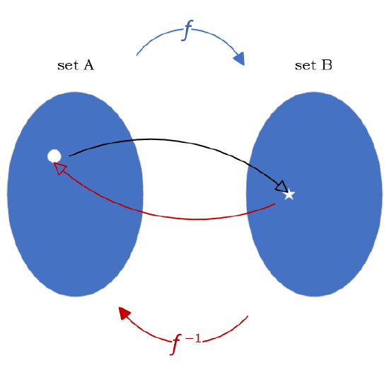
The solution is to look only at one-to-one functions. When a function is one-to-one, there is no ambiguity about which original input resulted in the output \(f(x)\). With the mapping visualization of functions, the picture below shows these cases.

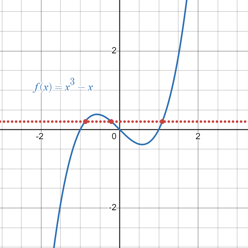
There is a handy dandy trick for assessing at a glance whether a function is one-to-one, using its graph.
If there is any place on the graph of a function where you can draw a horizontal line intersecting the graph multiple times, then it is not one-to-one.
A horizontal line has the equation \(y = a\) passing through some point \(a\) on the \(y\)-axis. If a graph intersects with this line, it means there is some point \( (x,a) \) where input \(x\) is sent to \(f(x) = a\). If there are multiple such points, \( (x_1,a)\) and \( (x_2, a) \), that means there are two inputs sent to the same output. For example, we already realized that \(f(x) = x^2\) is a problematic fave. We can see from his graph that he fails the Horizontal Line Test.

Tell whether each graphed function is one-to-one or not.
 |
.png?revision=1) |
 |
 |
| 1. | 2. | 3. | 4. |
- Answer
-
1. Yes, passes HLT 2. No, fails HLT 3. Yes, passes HLT 4. No, fails HLT 


Inverse Functions
Let \(f\) be a one-to-one function with domain \(A\) and range \(B\). Then its inverse function \(f^{-1}\) has domain \(B\) and range \(A\), and its values are defined by
\[ f^{-1}(y) = x \quad \text{ if and only if } \quad f(x) = y \notag \]
where \(y\) is in \(B\). This means that
\[ (f^{-1} \circ f)(x) = f^{-1}(f(x)) = x \quad \text{ and } \quad (f \circ f^{-1})(y) = f( f^{-1}(y)) = y \notag \]
for any \(x\) in \(A\), and any \(y\) in \(B\).
We also say that two functions with this relationship are inverses of each other. That is, the inverse of \(f^{-1}\) is \(f\). In math notation, this is the statement \( (f^{-1})^{-1} = f \).
In English, the inverse function takes an element \(y\) from \(B\) as input, and the function value it spits out will be the element from \(A\) that \(f\) had mapped to \(y\). Since \( f(x) = y\) is sometimes called the image of \(x\) under \(f\), you might hear \(x\) called a preimage of \(y\).
Given the following table representation of a function,
| \( x\) | \( f(x) \) |
| 0 | 0 |
| 1 | 2 |
| 2 | 4 |
| 3 | 6 |
find \( f^{-1}(0), f^{-1}(2), f^{-1}(4),\) and \( f^{-1}(6) \).
Solution
To find inverse function values, we just look backwards on each row of the table. So
- \( f^{-1}(0) = 0\)
- \( f^{-1}(2)=1\)
- \( f^{-1}(4)= 2\)
- \( f^{-1}(6) = 3 \)
The function from the table looks like \(f(x) = 2x \), "multiply something by 2," and we notice that the inverse function looks like the rule "divide something by 2," aka \( f^{-1}(x) = \frac{x}{2} \). This checks out, because the inverse operation of multiplication is division.
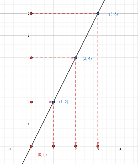
Given the graphed function \( f(x),\) find the values \( f^{-1}(0), f^{-1}(2), f^{-1}(4),\) and \( f^{-1}(6) \).

Solution
To read the values of the inverse function off of a graph of \(f\), just start with the \(y\)-value of interest, track it over to the graph, and then track downward to the \(x\)-axis to see which input value went with him. This is the same function as the previous example, so use the graph to confirm the answers.
Confirm algebraically that \(f(x) = 2x + 1 \) and \(f^{-1}(x) = \dfrac{x-1}{2} \) are inverses of each other.
Solution
The domain and range of both of these functions is \( \mathbb{R}\). We want to confirm that these functions undo each other by checking that \( (f^{-1} \circ f)(x) = x\) and \( (f\circ f^{-1})(x) = x\), for all real numbers \(x \). We compute:
\[ (f^{-1} \circ f)(x) = f^{-1}(f(x)) = f^{-1}(2x + 1) = \frac{ (2x+1) - 1}{2} = \frac{2x}{2} = x \quad \checkmark \notag \]
\[ (f\circ f^{-1})(x) = f( f^{-1}(x)) = f\left( \frac{x-1}{2} \right) = 2 \left( \frac{x-1}{2} \right) + 1 = x-1 + 1 = x \quad \checkmark \notag \]
Confirm algebraically that \( f(x) = x^3 \) and \( f^{-1}(x) = x^{\frac{1}{3}} \) are inverses of each other.
- Answer
-
For all \(x\) in \(\mathbb{R}\),
\[ (f^{-1} \circ f)(x) = f^{-1}(x^3) = (x^3)^{\frac{1}{3}} = x \quad \checkmark \notag \]
\[ (f\circ f^{-1})(x) = f( x^{\frac{1}{3}}) = (x^{\frac{1}{3}})^3 = x \quad \checkmark \notag \]
Given a particular function, how do you systematically figure out its inverse function? Follow this process:
To find the inverse of a function \(f (x)\),
- Write \(y = f(x)\), aka replace the left hand side of the function definition with "\(y\)."
- Solve this equation for \(x\) in terms of \(y\), if possible.
- Swap the variable names: replace all the \(x\)'s with \(y\)'s and vice versa.
- Replace \(y\) with "\(f^{-1}(x)\)."
Find the inverse function, if possible.
- \(f(x) = 4x -3 \)
- \( f(x) = \dfrac{ x+1}{x-1} \)
- \( f(x) = (x+4)^2 \)
Solution
1. Write \( y = 4x - 3 \). We solve this equation for \(x\) in terms of \(y\), getting \(x = \dfrac{y+3}{4} \). Now we swap all the \(x\)'s and \(y\)'s to get \(y = \dfrac{x+3}{4} \). We report the final answer as \( f^{-1}(x) = \dfrac{x+3}{4} \).
2. Write \( y = \dfrac{ x+1}{x-1} \). We start solving this equation for \(x\)...
\[ y = \dfrac{ x+1}{x-1} \quad \rightarrow \quad y(x-1) = x+1 \quad \rightarrow \quad xy - y = x+ 1 \notag \]
At this point, bring all the \(x\) terms to one side and everything else to the other.
\[ xy - x = y + 1 \quad \rightarrow \quad x(y - 1) = y+ 1 \quad \rightarrow \quad x = \dfrac{ y+1}{y-1} \notag \]
Swapping the variable names, we have \( y = \dfrac{ x+1}{x-1} \), so the final answer is \( f^{-1}(x) = \dfrac{ x+1}{x-1} \).
3. We write \(y = (x+4)^2 \) and start trying to solve for \(x\). The first thing we try to do is get rid of the power of 2...but when we do that, we get some ambiguity!
\[ x+4 = \pm \sqrt{y} \notag \]
We can't get an inverse to this function! If we graphed this function, it would fail the HLT.
Find the inverse function, if possible.
- \(f(x) = x^3 + 2 \)
- \( f(x) = \dfrac{ 2x+1}{x-3} \)
- \( f(x) =-2x^2 \)
- Answer
-
1. \( f^{-1}(x) = \sqrt[3]{x-2} \)
2. \( f^{-1}(x) = \dfrac{3x+1}{x-2} \)
3. This function has no inverse. I run into an issue when I try to take a square root to undo the square on the \(x\).
Let's wrap up by noticing something interesting about the graphs of inverse functions. Below, I've graphed some functions together with their inverse functions on the same coordinate planes, as well as a supplementary dotted line \(y = x\). What do you observe?

The graphs of inverse functions look like mirror images of each other when reflected over the line \(y = x\). Niftyyyyy. Look at the first graph and find the point \( (2,5)\) on the black line. That set of coordinates is telling us that \( f(2) = 5 \). We know that the inverse function must then satisfy \( f^{-1}(5) = 2 \). Oh but wait, that means that the point \( (5,2) \) should appear on the graph of \(f^{-1}\)! Look at the blue line. It does indeed pass through the point \( (5,2) \). Math! Still undefeated.
Okay, that's the scoop on inverses. Check out the exercises section to see some real-world applications like the one below!
Back in Section 4.1, we saw a function \(A(r) = \pi r^2\), which calculates the area of a circle with radius \(r\) that I was cutting out of a piece of cardboard. In that physical context, we determined that the sensible domain for this function should be \( 0 \leq r \leq 6\). Find the range for this function. Then find the inverse function giving the radius needed for a particular area value. Then determine the domain and range of the inverse function.
Solution
The area will increase as the radius increases, so the smallest area is found using the smallest possible radius, \(r = 0\) giving \(A = 0\), and the largest area is found using the largest possible radius, \(r = 6\) giving \(A = 36\pi \). Thus the function values that are actually attained are the range \( 0 \leq A \leq 36\pi\). The inverse function will have that set as its domain, and we think of it as taking area values as inputs and returning the radius that would be needed to achieve that area. We can go about this using the method above, with a few notational changes that just make sense.
Write \(A = \pi r^2\) and solve this equation for \(r\). As we go along, we reach a point where we take a square root, which normally is a red flag.
\[ A = \pi r^2 \quad \rightarrow \quad r^2 = \frac{A}{\pi} \quad \rightarrow \quad r = \pm \sqrt{\frac{A}{\pi}} \notag \]
Except!!! In this example, the domain of \(A(r)\) did NOT include negative numbers! So we actually have no ambiguity here, we are only taking the positive root. We have \( r = \sqrt{\frac{A}{\pi}} \).
Now, here I'm going to deviate a little bit from the process described above. I don't want to swap the variable names, because these letters were chosen to describe actual real-life quantities. I want to keep calling area values \(A\) and radius values \(r\). But I can indicate that I'm now seeing radius as a function of area by giving the answer \(r(A) = \sqrt{\frac{A}{\pi}} \). The range of this function will match the domain of the original, \( 0 \leq r \leq 6\).
These notational changes make it easy to know how to use this function later. Say I need a circle with area \( 4\pi \) square inches. I just plug that area value into my new function to get \( r(4\pi) = \sqrt{ \frac{4\pi}{\pi}} = 2\) inches.
* (Minecraft hopper image from Minecraft Wiki)