6.4 Basics of Logarithmic Functions

Learning Objectives

By the end of this section, you will be able to:

• recognize logarithmic functions, their important features, and their graphs
• relate logarithms to exponentials
• use logarithm laws to expand and condense logarithmic expressions
• evaluate logarithmic functions and use technology to solve problems

In the exercises section you just finished, I snuck in a certain type of question. I asked something like, "If \(f(x) = 9^x\), what does \(x\) need to be in order to make \(f(x) = 3\)?" In other words, I want to have \( 9^x = 3 \), and I wonder what \(x\) will make that true? Wait... 3 is the square root of 9, and we write roots with fractional exponents. So \(x = \frac{1}{2} \) will work! We can check: \( f\left( \frac{1}{2} \right) = 9^{\frac{1}{2}} = \sqrt{9} = 3 \).

Logarithms, at the end of the day, are just the way we deal with that question-and-answer process. You can also think of them as a way to undo the "raising to a power" process that happens inside an exponential equation. We've already learned that functions that undo other functions are called inverse functions. If you forgot that stuff, review Section 4.4.

Every exponential function \(f(x) = a^x\) (with \(a > 0\) and \(a \neq 1\)) passes the Horizontal Line Test and is thus one-to-one. Therefore, it has an inverse function \(f^{-1} \). Recall that being an inverse function means that the values \( f^{-1}(x) \) are defined by

\[ f^{-1}(x) = y \quad \iff \quad f(y) = x. \notag \]

Aka, if you want to know what \(f^{-1}(x) \) spits out, it's the number \(y\) such that \(f(y) = x\).

Logarithmic Functions

For \(a > 0\) and \( a \neq 1\), the logarithmic function with base \(a\), which we denote \( \log_a\), is the inverse function of the exponential function with the same base \(a\). Thus, it is defined by the relationship

\[ \log_a x = y \quad \iff \quad a^y = x. \tag{\(\star\)} \]

We say, "log base \(a\) of \(x\) is \(y\)." Basically, "\( \log_a (x) = ?\)" is asking the question, "What do I need to raise the base \(a\) to in order to get out this \(x\)?" The answer to that question is the output of the function \( \log_a\).

When in particular the base is the special number \(e\), we write \( \log_e x \) as \( \ln x\), and call it the natural log of \(x\).

Fun facts about logarithmic functions:

• Their domain is only positive real numbers! You are not allowed to put 0 or a negative number into a log, because that would be the same as saying \( a^{y} = 0 \), and there's no possible \(y\) that will satisfy that!
• Since \(a^0 = 1\) for any \(a\), we have \( \log_a (1) = 0\) for any base \(a\). This is something you should know without using a calculator.
• Similarly, since \(a^1 = a \), we have \( \log_a(a) = 1\) for any \(a\). Aka, if you take the log of its own base, you will always get 1. This is the other evaluation you should know without a calculator.

The fact that \(a\) is called the base in both equations where it appears should help you remember that \(\log_a\) is related to \(a^x\). Whenever the input for a log function might be ambiguous, you can use parentheses; for example, \(\log_a(x+1) \) tells you \((x+1)\) is the whole input, whereas \( \log_a x + 1 \) would be interpreted as "compute \( \log_a \) of \(x\) and then add 1 to the result."

I just want to emphasize again that the relationship \((\star)\) in the definition above is your bread and butter here. You will generally always be translating back and forth between these two forms whenever working with logarithms in functions or equations. Memorize that guy!!!

Now let's see what these functions look like. Recall that the graphs of inverse functions look like mirror images, reflected across the diagonal line \(y = x\). This means that to remember what the graphs of logarithmic functions look like, you just have to remember exponential graphs and then reflect them. The beautiful thing about math is that you don't have to memorize a bunch of random stuff. You can just memorize a few things and then deduce the rest from them!

Study the graphs below and see if you can detect any patterns and observations.

Observations:

• While exponential functions exhibited fast growth (or decay), logarithmic functions exhibit slow growth (or decay).
• They all pass through the point \( (1,0)\), which makes sense because \( \log_a ( 1) = 0 \), as mentioned in the fun facts.
• Looking closely, you can see each one pass through \( (a, 1)\) for its base. Example: \( f(x) = \log_{10}(x)\) passes through \((10, 1)\).
• They all have a vertical asymptote \( x = 0\). Aka, they never touch or cross over the \(y\)-axis, because their domain is only defined for \(x > 0\).
• If \(a > 1\), the function is increasing (going uphill). If \( 0 < a < 1\), the function is decreasing.
• Notice that \( p(x)\) is the reflection of \( f(x)\) over the \(x\)-axis, and their bases are reciprocals. This will always happen.
• I've included on this graph the Big Guys that your science professors asked me to cover. Mostly people use base 10 and base \(e\) (the natural log) and you'll find these buttons on a calculator. Computer science uses a log of base 2, in a shock to no one.
• Looking out at end behavior, so for \(x \rightarrow \infty \), we see that the bigger the base, the slower the growth. Thus you see since \( 2 < e < 10\), the graph of \(\ln x\) lies between the graphs of \( \log_{10} x \) and \( \log_2 x \).

We should also make sure we understand what it means for exponential and logarithmic functions to be inverses. Let's discuss and then summarize. First, consider what happens if we plug an input \(x\) into an exponential function, and then apply the corresponding logarithm, by definition:

\[ \log_a (a^x) = ? \quad \iff \quad a^? = a^x \notag \]

Oh, duh. We must have \(? = x\) to make the translated equation true. So doing an exponential and then a log gives you back the original input. Next, consider the other direction of composition, by definition:

\[ a^{\log_a x} = ? \quad \iff \quad \log_a (?) = \log_a (x) \notag \]

Aha, again we must have \(? = x\) to make the translation true. So doing a log and then the corresponding exponential gives you back the original input. Inverse relationship confirmed!

\[ \log_a (a^x) = x, \: \text{ for all real numbers } x \quad \text{ and } \quad a^{\log_a x} = x, \: \text{ for all } x> 0 \notag \]

Test your understanding with the exercises below.

Exercise \(\PageIndex{1}\)

Answer True/False.

1. For \( f(x) = \log_{2}(x) \), we have \( f(4) = 2 \).
2. For \( f(x) = \log_2 (x) \), we have \( f\left(\frac{1}{2}\right) = -1 \).
3. For \( f(x) = \log_{10}(x) \), we have \( f(1) = 100 \).
4. I am allowed to plug in \(x = 0\) to the function \(f(x) = \ln x\).
5. I am allowed to plug in \(x = 1 \) to the function \( f(x) = \ln x \).
6. I am allowed to plug in \(x = 1\) to the function \( f(x) = \ln (x-1) \).
7. The graph of the function \(f(x) = \log_2 x \) is the reflection of \( g(x) = 2^x\) across the \(y\)-axis.
8. The graph of the function \( f(x) = \log_2 x \) is the reflection of \(g(x) = 2^x\) across the line \(y = x\).
9. The graph of the function \( f(x) = \log_{1/2} x \) is the reflection of \(g(x) = \log_2 x\) across the \(x\)-axis.
10. The graph of \(f(x) = \log_3 x\) passes through \( (1,0) \).
11. The graph of \(f(x) = \log_3 x\) passes through \( (0,1) \).
12. The graph of \(f(x) = \log_3 x\) passes through \( (3,1) \).
13. The graph of \(f(x) = \log_a x\) passes through \( (a,1) \).
14. For \(f(x) = e^x\) and \(g(x) = \ln x\), we know \( (f \circ g)(x) = x \), for all \(x > 0\).
15. As \(x \rightarrow \infty\), the graph of \( f(x) = \log_{5} x \) exhibits slower growth (is less steep) than \( g(x) = \ln x \), for \( x > 1\).
16. \( \ln (x) > \log_5 x \) for \(x > 1\).
17. As \(x \rightarrow \infty\), the graph of \( f(x) = \log_5 x \) exhibits faster growth (is steeper) than \( g(x) = \log_{10} x \), for \( x > 1\).

Answer

1. True, we translate \( f(4) = \log_2(4) = ?\) to \( 2^? = 4 \) and see that it must give the answer \( 2\).
2. True, we translate \( f\left(\frac{1}{2}\right) = \log_2 \left( \frac{1}{2} \right) = ?\) to \( 2^? = \frac{1}{2} \) and see that the power must be \(-1\).
3. False, we translate \( \log_{10}(1) = ?\) to \( 10^? = 1\) and see that the power must be \(0\), not \(100\). Or just remember that for any base, the log of 1 is 0.
4. False, we can't plug 0 into any logs.
5. True, \(x = 1\) is in the domain.
6. False, plugging in \(x = 1\) results in plugging in \( 1-1 = 0\) into the log, which is illegal.
7. False, these are inverse functions, so the graphs are reflections across the line \(y = x\).
8. True.
9. True, we observed that above.
10. True, all such logs pass through \( (1,0)\).
11. False, we can't even plug in the \(x\)-value 0.
12. True, if we plug in \(x = 3\), we are taking the log of its own base, which gives 1.
13. True, this always works.
14. True, since \( \ln\) means log base \(e\), these are inverse functions.
15. True, the bigger the base, the slower the growth, and \(5 > e\).
16. True, slower growth means that at some \(x\)-value like \(x = 2\), the graph of \( \log_5 x \) will be lower than the graph of \( \ln x\), so has a smaller function value.
17. True, the bigger the base, the slower the growth, so base 5 is faster growing than base 10.

Exercise \(\PageIndex{2}\)

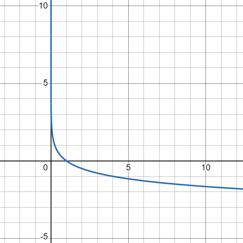
Match the graphs to their functions.

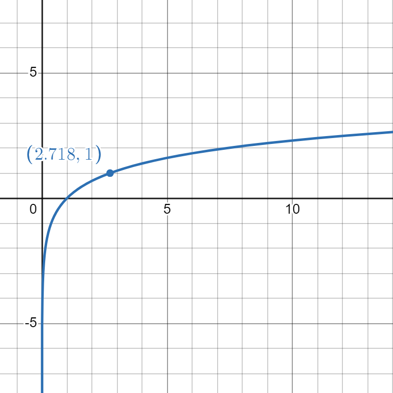1.	2.	3.	4.
\( f(x) = \ln x \)	\( g(x) = \log_{10} x \)	\( h(x) = \log_3 x \)	\( p(x) = \log_{0.25} x \)

Answer

1. This graph passes through \( (10, 1)\), so the base is 10 and goes with \(g\).
2. This graph passes through \( (3,1)\), so it goes with \(h\).
3. This graph must have a fractional base because it's descending, so it must go with \(p\). We can confirm by checking the point \( (4,-1)\) that the graph passes through. Indeed, \( \log_{0.25}(4) = ? \) translates to \( \left(\frac{1}{4}\right)^? = 4 \) and the function value must be \( -1\). Goes with \( p\).
4. Remember that \( e \approx 2.71...\) so that's the point being labeled. Must go with \(f\).

Log Laws

I want to briefly introduce you to the Logarithm Laws. These laws all follow from power rules (and if you're interested in going deeper into that, check out Chapter 7). These laws are used to expand and condense expressions containing logarithms. So they let us work with stuff like this:

\[ \log_2 (x) + \log_2 (x+1), \quad \quad \ln \left( \frac{x}{y} \right)^3, \quad \quad 3 \log_{10} x + 2 \log_{10} x - \log_{10} (10x) \notag \]

These types of expressions must be dealt with in courses like Calc I and Calc II for sure. Let's get right into them.

Log Law	English Translation	Caveman Translation
\( \log_a (AB) = \log_a A + \log_a B \)	The logarithm of a product of expressions (numbers, variables, whatever as long as it is being multiplied) is the sum of the logarithms of the expressions.	Multiplication inside the log can be written as addition outside the log. Used backwards, addition outside the log translates to multiplication inside the log.
\( \log_a \left( \frac{A}{B} \right) = \log_a A - \log_a B \)	The logarithm of a quotient of expressions is the difference of the logarithms of the expressions.	Division inside the log can be written as subtraction outside the log. Used backwards, subtraction outside the log translates to division inside the log. The denominator must be the input whose log term is subtracted!
\( \log_a ( A^B) = B \log_a A \)	The logarithm of an expression raised to a power is the power times the logarithm of the expression.	If the whole input is raised to a power, you can bring powers down in front as coefficients.

Note: The bases must match in order to use these laws backwards! Using them forwards is called expanding, and using them backwards is called condensing. These laws are remixed to deal with big complicated combo expressions as well.

Example \(\PageIndex{1}\)

Expand fully or condense fully. Simplify if reasonable.

1. \( \log_2( xy) \)
2. \( \log_2 ( 2xyz) \)
3. \( \ln \left( \frac{ 1}{x} \right) \)
4. \( \ln ( x^3 y^5 ) \)
5. \( 2\log_5 x - \log_5 x \)
6. \( \ln A - \ln B + \ln C - \ln D \)
7. \( 3 \log_3 x + 2 \log_3 y \)

Solution

1. We expand \( \log_2(xy) = \log_2 x + \log_2 y \).

2. We split all the multiplications using additions outside the logs: \( \log_2(2xyz) = \log_2 (2) + \log_2 x + \log_2 y + \log_2 z \). We also simplify the \( \log_2 (2) \) term while we're at it, to get \( 1 + \log_2 x + \log_2 y + \log_2 z \).

3. We expand \( \ln \left( \frac{ 1}{x} \right) = \ln 1 - \ln x \) and simplify since any log with 1 plugged in will give 0, to get \( - \ln x \). By the way, you could get straight here by remembering that \( \frac{1}{x} = x^{-1} \) and using the bring powers down rule...

4. We expand and bring the powers down to get \( \ln ( x^3 y^5 ) = \ln x^3 + \ln y^5 = 3 \ln x + 5 \ln y \). Note that we cannot write \( (3)(5)(\ln xy) \) because the entire input must be raised to a single power in order to bring that power down in front!

5. We're condensing now. First move any coefficients up as powers, then condense any additions or subtractions. We get \( \log_5 x^2 - \log_5 x = \log_5 \left( \frac{x^2}{x} \right) = \log_5 (x) \). You can also get straight here by recognizing that \( 2A - A = A\) no matter how ugly \(A\) is.

6. Any additions get multiplied, and any subtractions get divided, so just sort them between the numerator and denominator of a fraction in the input! We get \( \ln \left(\frac{AC}{BD} \right) \).

7. Bring powers up first and then condense! We get \( \log_3 x^3 + \log_3 y^2 = \log_3 (x^3 y^2) \).

Exercise \(\PageIndex{3}\)

Expand fully or condense fully. Simplify if reasonable.

1. \( \ln[(x+3)(x-1)] \)
2. \( \log_{10} \left( \frac{ 10x}{y} \right) \)
3. \( \log_2 (2x^2 y^3 ) \)
4. \( \ln x + \ln y - 3 \ln z \)
5. \( 4 \log_3 (A+1) - 2 \log_3 (B ) \)

Answer

1. \( \ln (x+3) + \ln(x-1) \)

2. \( 1 + \log_{10} x - \log_{10} y \)

3. \( 1 + 2 \log_2 x + 3 \log_2 y \)

4. \( \ln \left( \frac{ x y}{z^3} \right) \)

5. \( \log_3 \left( \frac{ (A+1)^4}{B^2} \right) \)

Using Logarithms

Generally, you will need to use a calculator of some sort to deal with logarithm application problems. Here are some basic examples.

Example \(\PageIndex{2}\)

The age of an ancient object can be determined by seeing how much radioactive carbon-14 is left in it, because we know how fast carbon-14 dissipates as a substance ages. If we know the original amount of carbon-14 was \( C_0\), and we measure only \(C\) remaining, then we can calculate the age in years using the formula

\[ A = -8267 \ln \frac{C}{C_0} \notag \]

To avoid dealing with annoying numbers, let's say that whatever \(C_0\) was, I know that \(C\) is only 50% of it. (Using a calculator) find the age of the object. What if we're all the way down to 25% of the original amount?

Solution

If we're down to 50%, then in math terms we know \(C = 0.5 C_0\). We can plug this into the formula and simplify:

\[ A = -8267 \ln \frac{0.5 C_0}{C_0} = -8267 \ln (0.5) \notag \]

Using a calculator, we get about \(A = 5730\) years old. If \( C = 0.25 C_0 \) instead, we get

\[ A = -8267 \ln \frac{0.25 C_0}{C_0} = -8267 \ln (0.25) = 11,460 \text{ years} \notag \]

Example \(\PageIndex{3}\)

You will notice that since many populations exhibit exponential growth, many formulas for computations about populations will involve their inverse functions, logarithms. I had that Petri dish of bacteria, remember? It doubles in population every half hour, meaning that every half hour, each bacterium divides into two copies. I started with 200 bacteria, and it turns out that I can compute the amount of time (in hours) needed to reach \(N\) bacteria using the formula

\[ t = \frac{ \ln \frac{N}{200}}{2 \ln 2} \notag \]

Find how long it will take for me to have 800 bacteria, without using a calculator actually. Then using a calculator, find how long it will take to reach 1000 bacteria.

Solution

If you want to learn how to find that formula, check out Chapter 7. For now, let's just use it to compute:

\[ t = \frac{ \ln \frac{800}{200}}{2 \ln 2} = \frac{ \ln 4 }{2 \ln 2} \notag \]

Now you say, "I need my calculator!" No you don't! Notice that \( \ln 4 = \ln (2^2) \), right? Then use the bringing-down-powers rule...

\[ t = \frac{ 2\ln 2}{2 \ln 2} = 1 \text{ hour.} \notag \]

You can also just use common sense here... if I'm doubling every half hour and I notice that going from 200 to 800 is just doubling twice, then of course it will only take one hour!

To deal with \(N = 1000\), you can calculate:

\[ t = \frac{ \ln \frac{1000}{200}}{2 \ln 2} = \frac{ \ln 5}{2 \ln 2} \approx 1.161 \text{ hours.} \notag \]