6.4E Exercises

Last updated
Save as PDF

Page ID: 155607

$ \newcommand{\vecs}[1]{\overset { \scriptstyle \rightharpoonup} {\mathbf{#1}} } $

$ \newcommand{\vecd}[1]{\overset{-\!-\!\rightharpoonup}{\vphantom{a}\smash {#1}}} $

$ \newcommand{\id}{\mathrm{id}}$ $ \newcommand{\Span}{\mathrm{span}}$

( \newcommand{\kernel}{\mathrm{null}\,}\) $ \newcommand{\range}{\mathrm{range}\,}$

$ \newcommand{\RealPart}{\mathrm{Re}}$ $ \newcommand{\ImaginaryPart}{\mathrm{Im}}$

$ \newcommand{\Argument}{\mathrm{Arg}}$ $ \newcommand{\norm}[1]{\| #1 \|}$

$ \newcommand{\inner}[2]{\langle #1, #2 \rangle}$

$ \newcommand{\Span}{\mathrm{span}}$

$ \newcommand{\id}{\mathrm{id}}$

$ \newcommand{\Span}{\mathrm{span}}$

$ \newcommand{\kernel}{\mathrm{null}\,}$

$ \newcommand{\range}{\mathrm{range}\,}$

$ \newcommand{\RealPart}{\mathrm{Re}}$

$ \newcommand{\ImaginaryPart}{\mathrm{Im}}$

$ \newcommand{\Argument}{\mathrm{Arg}}$

$ \newcommand{\norm}[1]{\| #1 \|}$

$ \newcommand{\inner}[2]{\langle #1, #2 \rangle}$

$ \newcommand{\Span}{\mathrm{span}}$ $ \newcommand{\AA}{\unicode[.8,0]{x212B}}$

$ \newcommand{\vectorA}[1]{\vec{#1}} % arrow$

$ \newcommand{\vectorAt}[1]{\vec{\text{#1}}} % arrow$

$ \newcommand{\vectorB}[1]{\overset { \scriptstyle \rightharpoonup} {\mathbf{#1}} } $

$ \newcommand{\vectorC}[1]{\textbf{#1}} $

$ \newcommand{\vectorD}[1]{\overrightarrow{#1}} $

$ \newcommand{\vectorDt}[1]{\overrightarrow{\text{#1}}} $

$ \newcommand{\vectE}[1]{\overset{-\!-\!\rightharpoonup}{\vphantom{a}\smash{\mathbf {#1}}}} $

$ \newcommand{\vecs}[1]{\overset { \scriptstyle \rightharpoonup} {\mathbf{#1}} } $

$ \newcommand{\vecd}[1]{\overset{-\!-\!\rightharpoonup}{\vphantom{a}\smash {#1}}} $

$\newcommand{\avec}{\mathbf a}$ $\newcommand{\bvec}{\mathbf b}$ $\newcommand{\cvec}{\mathbf c}$ $\newcommand{\dvec}{\mathbf d}$ $\newcommand{\dtil}{\widetilde{\mathbf d}}$ $\newcommand{\evec}{\mathbf e}$ $\newcommand{\fvec}{\mathbf f}$ $\newcommand{\nvec}{\mathbf n}$ $\newcommand{\pvec}{\mathbf p}$ $\newcommand{\qvec}{\mathbf q}$ $\newcommand{\svec}{\mathbf s}$ $\newcommand{\tvec}{\mathbf t}$ $\newcommand{\uvec}{\mathbf u}$ $\newcommand{\vvec}{\mathbf v}$ $\newcommand{\wvec}{\mathbf w}$ $\newcommand{\xvec}{\mathbf x}$ $\newcommand{\yvec}{\mathbf y}$ $\newcommand{\zvec}{\mathbf z}$ $\newcommand{\rvec}{\mathbf r}$ $\newcommand{\mvec}{\mathbf m}$ $\newcommand{\zerovec}{\mathbf 0}$ $\newcommand{\onevec}{\mathbf 1}$ $\newcommand{\real}{\mathbb R}$ $\newcommand{\twovec}[2]{\left[\begin{array}{r}#1 \\ #2 \end{array}\right]}$ $\newcommand{\ctwovec}[2]{\left[\begin{array}{c}#1 \\ #2 \end{array}\right]}$ $\newcommand{\threevec}[3]{\left[\begin{array}{r}#1 \\ #2 \\ #3 \end{array}\right]}$ $\newcommand{\cthreevec}[3]{\left[\begin{array}{c}#1 \\ #2 \\ #3 \end{array}\right]}$ $\newcommand{\fourvec}[4]{\left[\begin{array}{r}#1 \\ #2 \\ #3 \\ #4 \end{array}\right]}$ $\newcommand{\cfourvec}[4]{\left[\begin{array}{c}#1 \\ #2 \\ #3 \\ #4 \end{array}\right]}$ $\newcommand{\fivevec}[5]{\left[\begin{array}{r}#1 \\ #2 \\ #3 \\ #4 \\ #5 \\ \end{array}\right]}$ $\newcommand{\cfivevec}[5]{\left[\begin{array}{c}#1 \\ #2 \\ #3 \\ #4 \\ #5 \\ \end{array}\right]}$ $\newcommand{\mattwo}[4]{\left[\begin{array}{rr}#1 \amp #2 \\ #3 \amp #4 \\ \end{array}\right]}$ $\newcommand{\laspan}[1]{\text{Span}\{#1\}}$ $\newcommand{\bcal}{\cal B}$ $\newcommand{\ccal}{\cal C}$ $\newcommand{\scal}{\cal S}$ $\newcommand{\wcal}{\cal W}$ $\newcommand{\ecal}{\cal E}$ $\newcommand{\coords}[2]{\left\{#1\right\}_{#2}}$ $\newcommand{\gray}[1]{\color{gray}{#1}}$ $\newcommand{\lgray}[1]{\color{lightgray}{#1}}$ $\newcommand{\rank}{\operatorname{rank}}$ $\newcommand{\row}{\text{Row}}$ $\newcommand{\col}{\text{Col}}$ $\renewcommand{\row}{\text{Row}}$ $\newcommand{\nul}{\text{Nul}}$ $\newcommand{\var}{\text{Var}}$ $\newcommand{\corr}{\text{corr}}$ $\newcommand{\len}[1]{\left|#1\right|}$ $\newcommand{\bbar}{\overline{\bvec}}$ $\newcommand{\bhat}{\widehat{\bvec}}$ $\newcommand{\bperp}{\bvec^\perp}$ $\newcommand{\xhat}{\widehat{\xvec}}$ $\newcommand{\vhat}{\widehat{\vvec}}$ $\newcommand{\uhat}{\widehat{\uvec}}$ $\newcommand{\what}{\widehat{\wvec}}$ $\newcommand{\Sighat}{\widehat{\Sigma}}$ $\newcommand{\lt}{<}$ $\newcommand{\gt}{>}$ $\newcommand{\amp}{&}$ $\definecolor{fillinmathshade}{gray}{0.9}$

Definition True/False

Answer True/False. If False, explain why.

If $ \log_a x = y $, then $ a^x = y $.
If $ \log_b a = c $, then $ b^c = a$.
There is a logarithmic function with base $1$, $ f(x) = \log_1 x $.
The natural log function $ \ln x$ is the logarithmic function with base $\pi$.
Let $f(x) = \log_a x $ be a logarithmic function ($ a> 0, a \neq 1 $). The domain of $f$ is $ \{ x \: | \: x \geq 0 \} $.
Let $f(x) = \log_a x $ be a logarithmic function ($ a> 0, a \neq 1 $). The domain of $f$ is $ \{ x \: | \: x > 0 \} $.
I am allowed to plug in $ x = -2$ to the function $ f(x) = \ln (x + 3 ) $.
I am allowed to plug in $ x = -2 $ to the function $ f(x)= \ln (x + 1) $.
For any base $a$, $\log_a(a) = 1$.
For any base $a$, $ \log_a(0) = 1$.
For any base $ a$, $ \log_a(1) = 0 $.
For $f(x) = \log_{10}x$ and $ g(x) = 10^x $, we know $ (g \circ f) (x) = x$ for all $x>0$.

Answer

F, this does not match the definition. It must be $a^y = x$.
T
F, we do not allow the base $a = 1$. (Why doesn't it make sense?)
F, it's base $e$.
F, we can't have $\geq$ because 0 is not allowed.
T
T
F, if $x = -2$ then the input to the log is $ -2 + 1 = -1$, a negative number.
T
F, 0 isn't even in the domain.
T
T

Graphs True/False

Answer True/False. If False, justify or find the error.

The graph of $ f(x) = \log_3 x $ passes through $ (1,0)$.
The graph of $ f(x) = \log_a x $ passes through $ (1,a)$ for any base $a$.
The graph of $ f(x) = \log_a x $ passes through $ (a,1)$ for any base $a$.
The graph of the function $ f(x) = \log_3 x $ is the reflection of the graph of $g(x) = \log_{\frac{1}{3}} x $ across the $x$-axis.
The graph of the function $f(x) = \ln x $ is the reflection of the graph of $ g(x) = e^x $ across the $x$-axis.
The graph of $ f(x) = \log_2 x $ exhibits faster growth than the graph of $ g(x) = \ln x$, for $x > 1$.
The graph of $ f(x) = \log_{10} x $ exhibits faster growth than the graph of $ g(x) = \ln x$, for $x > 1$.

Answer

T
F, it passes through $ (1,0)$.
T
T
F, it's the reflection across the line $ y = x$ because they're inverse functions.
T
F, the base $10 > e$.

Matching Graphs

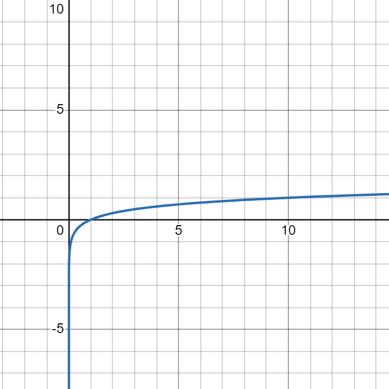
By analyzing signal points like $ (a,1)$ and using your knowledge of logarithmic function graphs, match the graphs to their functions.

$log6.png$	$log4.png$	$log1.png$	$log5.png$
1.	2.	3.	4.
$ f(x) = \log_{10} x $	$ g(x) = \ln x$	$ h(x) = \log_{\frac{1}{2}} x $	$ p(x) = \log_2 x $

Answer

$p$
$g$
$f$
$h$

Working With Logarithms

Without using a calculator, compute the following using the definition and Log Laws:

$ \log_3 9$
$ \log_{17}(1) $
$ \log_2 \left( \frac{1}{4} \right) $
$ \ln e $
$ \ln e^4 $
$ \log_{10} 1000 $
$ \log_2 4 + 2 \log_2 8 $
$ \log_3 (6) - \log_3 ( 2) $

Answer

$2$
$0$
$ -2$
$ 1$
$ 4$
$ 3$
$8$
$ 1$ (Hint: consider $ \log_3(6) = \log_3(2 \cdot 3) $.)

Condensing/Expanding

Fully expand or fully condense. Simplify if reasonable.

$ \log_2 \left( \frac{ x}{2} \right) $
$ \log_{10} (100x^2y^3) $
$ \ln (A^2 + 2AB + B^2) $
$ \log_3 11 + \log_3 7 $
$ \ln x + \ln y - 2 \ln z - 3 \ln (w+1) $
$ 3 \log_a (A+B) - 4 \log_a (A -B) $

Answer

$ \log_2 x - 1 $
$ 2 + 2 \log_{10} x + 3 \log_{10} y $
$ 2 \ln (A+B) $
$ \log_3 (77) $
$ \ln \left( \dfrac{x y}{z^2 (w+1)^3} \right) $
$ \log_a \left( \dfrac{ (A+B)^3}{(A-B)^4} \right) $

Logarithms Vs. Exponentials True/False

Answer True/False. Justify your answer.

$ \log_2( 2^x) = x $
$ \log_2( 8) = 3 $
For any base $ a$, $ \log_a (x^a) = x $.
$ e^{\ln x} = x $ (for $x > 0 $
$ e^{ \log_{10} x} = x $ (for $x > 0 $
$ 10^{ \log_{10}x } = x $ (for $x > 0 $

Answer

T, inverse functions.
T, write as $ \log_2 (2^3) = 3 \log_2 2$ or translate with definition.
F, it should be $ \log_a (a^x) = x$.
T, inverse functions.
F, the bases must match.
T, inverse functions.

Applications

1. We saw how exponential functions can be used to calculate interest compounding annually. In fact, you can choose to compound multiple times a year, or even continuously. For continuously compounding interest, the amount of money you have at time $t$ years after investing an initial amount $A_0$ is given by $A = A_0 e^{rt} $, where $r$ is the interest rate written as a decimal. Say I want to double my money, so that $A$ is $ 2A_0$. Then my equation becomes $ 2 = e^{rt} $. Give the equivalent logarithmic equation. Solve it for $t$. If the interest rate is 12%, find the time $t$ it will take to double my money. (Use a calculator if needed.)

2. If I take a turkey out of the oven with internal temperature $165^\circ $F and place it in an ambient room temperature of $65^\circ$F, then the amount of time (in minutes) it will take to cool to an internal temperature of $T$ is given by

\[ t = -40 \ln \left( \frac{T-65}{100} \right) \notag \]

Use a calculator to find how long it takes to cool down to $150^\circ$F, $125^\circ$F, and $100^\circ$F.

Answer

1. The equivalent equation is $ \ln (2) = rt $. Solved for $t$, we have $ t = \frac{ \ln 2}{r} $. If $r = .12$, then $t \approx 5.78$ years.

2. For $T = 150^\circ$F, $ t \approx 6.5$ minutes. For $T =125^\circ$F, $ t \approx 20.4$ minutes. For $ T = 100^\circ$F, $t \approx 42$ minutes.

Search

Text Color

Text Size

Margin Size

Font Type