6.3 Basics of Exponential Functions

Last updated
Save as PDF

Page ID: 155422

$ \newcommand{\vecs}[1]{\overset { \scriptstyle \rightharpoonup} {\mathbf{#1}} } $

$ \newcommand{\vecd}[1]{\overset{-\!-\!\rightharpoonup}{\vphantom{a}\smash {#1}}} $

$ \newcommand{\id}{\mathrm{id}}$ $ \newcommand{\Span}{\mathrm{span}}$

( \newcommand{\kernel}{\mathrm{null}\,}\) $ \newcommand{\range}{\mathrm{range}\,}$

$ \newcommand{\RealPart}{\mathrm{Re}}$ $ \newcommand{\ImaginaryPart}{\mathrm{Im}}$

$ \newcommand{\Argument}{\mathrm{Arg}}$ $ \newcommand{\norm}[1]{\| #1 \|}$

$ \newcommand{\inner}[2]{\langle #1, #2 \rangle}$

$ \newcommand{\Span}{\mathrm{span}}$

$ \newcommand{\id}{\mathrm{id}}$

$ \newcommand{\Span}{\mathrm{span}}$

$ \newcommand{\kernel}{\mathrm{null}\,}$

$ \newcommand{\range}{\mathrm{range}\,}$

$ \newcommand{\RealPart}{\mathrm{Re}}$

$ \newcommand{\ImaginaryPart}{\mathrm{Im}}$

$ \newcommand{\Argument}{\mathrm{Arg}}$

$ \newcommand{\norm}[1]{\| #1 \|}$

$ \newcommand{\inner}[2]{\langle #1, #2 \rangle}$

$ \newcommand{\Span}{\mathrm{span}}$ $ \newcommand{\AA}{\unicode[.8,0]{x212B}}$

$ \newcommand{\vectorA}[1]{\vec{#1}} % arrow$

$ \newcommand{\vectorAt}[1]{\vec{\text{#1}}} % arrow$

$ \newcommand{\vectorB}[1]{\overset { \scriptstyle \rightharpoonup} {\mathbf{#1}} } $

$ \newcommand{\vectorC}[1]{\textbf{#1}} $

$ \newcommand{\vectorD}[1]{\overrightarrow{#1}} $

$ \newcommand{\vectorDt}[1]{\overrightarrow{\text{#1}}} $

$ \newcommand{\vectE}[1]{\overset{-\!-\!\rightharpoonup}{\vphantom{a}\smash{\mathbf {#1}}}} $

$ \newcommand{\vecs}[1]{\overset { \scriptstyle \rightharpoonup} {\mathbf{#1}} } $

$ \newcommand{\vecd}[1]{\overset{-\!-\!\rightharpoonup}{\vphantom{a}\smash {#1}}} $

$\newcommand{\avec}{\mathbf a}$ $\newcommand{\bvec}{\mathbf b}$ $\newcommand{\cvec}{\mathbf c}$ $\newcommand{\dvec}{\mathbf d}$ $\newcommand{\dtil}{\widetilde{\mathbf d}}$ $\newcommand{\evec}{\mathbf e}$ $\newcommand{\fvec}{\mathbf f}$ $\newcommand{\nvec}{\mathbf n}$ $\newcommand{\pvec}{\mathbf p}$ $\newcommand{\qvec}{\mathbf q}$ $\newcommand{\svec}{\mathbf s}$ $\newcommand{\tvec}{\mathbf t}$ $\newcommand{\uvec}{\mathbf u}$ $\newcommand{\vvec}{\mathbf v}$ $\newcommand{\wvec}{\mathbf w}$ $\newcommand{\xvec}{\mathbf x}$ $\newcommand{\yvec}{\mathbf y}$ $\newcommand{\zvec}{\mathbf z}$ $\newcommand{\rvec}{\mathbf r}$ $\newcommand{\mvec}{\mathbf m}$ $\newcommand{\zerovec}{\mathbf 0}$ $\newcommand{\onevec}{\mathbf 1}$ $\newcommand{\real}{\mathbb R}$ $\newcommand{\twovec}[2]{\left[\begin{array}{r}#1 \\ #2 \end{array}\right]}$ $\newcommand{\ctwovec}[2]{\left[\begin{array}{c}#1 \\ #2 \end{array}\right]}$ $\newcommand{\threevec}[3]{\left[\begin{array}{r}#1 \\ #2 \\ #3 \end{array}\right]}$ $\newcommand{\cthreevec}[3]{\left[\begin{array}{c}#1 \\ #2 \\ #3 \end{array}\right]}$ $\newcommand{\fourvec}[4]{\left[\begin{array}{r}#1 \\ #2 \\ #3 \\ #4 \end{array}\right]}$ $\newcommand{\cfourvec}[4]{\left[\begin{array}{c}#1 \\ #2 \\ #3 \\ #4 \end{array}\right]}$ $\newcommand{\fivevec}[5]{\left[\begin{array}{r}#1 \\ #2 \\ #3 \\ #4 \\ #5 \\ \end{array}\right]}$ $\newcommand{\cfivevec}[5]{\left[\begin{array}{c}#1 \\ #2 \\ #3 \\ #4 \\ #5 \\ \end{array}\right]}$ $\newcommand{\mattwo}[4]{\left[\begin{array}{rr}#1 \amp #2 \\ #3 \amp #4 \\ \end{array}\right]}$ $\newcommand{\laspan}[1]{\text{Span}\{#1\}}$ $\newcommand{\bcal}{\cal B}$ $\newcommand{\ccal}{\cal C}$ $\newcommand{\scal}{\cal S}$ $\newcommand{\wcal}{\cal W}$ $\newcommand{\ecal}{\cal E}$ $\newcommand{\coords}[2]{\left\{#1\right\}_{#2}}$ $\newcommand{\gray}[1]{\color{gray}{#1}}$ $\newcommand{\lgray}[1]{\color{lightgray}{#1}}$ $\newcommand{\rank}{\operatorname{rank}}$ $\newcommand{\row}{\text{Row}}$ $\newcommand{\col}{\text{Col}}$ $\renewcommand{\row}{\text{Row}}$ $\newcommand{\nul}{\text{Nul}}$ $\newcommand{\var}{\text{Var}}$ $\newcommand{\corr}{\text{corr}}$ $\newcommand{\len}[1]{\left|#1\right|}$ $\newcommand{\bbar}{\overline{\bvec}}$ $\newcommand{\bhat}{\widehat{\bvec}}$ $\newcommand{\bperp}{\bvec^\perp}$ $\newcommand{\xhat}{\widehat{\xvec}}$ $\newcommand{\vhat}{\widehat{\vvec}}$ $\newcommand{\uhat}{\widehat{\uvec}}$ $\newcommand{\what}{\widehat{\wvec}}$ $\newcommand{\Sighat}{\widehat{\Sigma}}$ $\newcommand{\lt}{<}$ $\newcommand{\gt}{>}$ $\newcommand{\amp}{&}$ $\definecolor{fillinmathshade}{gray}{0.9}$

↵

Learning Objectives

By the end of this section, you will be able to:

recognize exponential functions, their important features, and their graphs
evaluate exponential functions and use technology to solve problems

We can raise numbers to powers in our sleep at this point, but mostly we've done integer and rational powers. That is, you see stuff like $4^2, 9^{\frac{1}{2}}, 100^{-2} $ without having an allergic reaction (hopefully). But what would you do if I jump out the bushes and throw a $ 3^\pi $ across your path?? We've basically ignored a whole set of real numbers as power options—the irrational numbers. Stuff like

\[ 2^\pi, \quad 5^{\sqrt{2}}, \quad 8^e. \notag \]

Until today! The way we deal with irrational powers is to approximate them with rational powers till you're "close enough" that any error is irrelevant for your purposes. We use calculators to do this, don't worry! Remember that we can approximate $ \pi \approx 3.14159... $, $ \sqrt{2} \approx 1.414213... $, and $e \approx 2.718281...$. A calculator can then evaluate

\[ 2^\pi \approx 8.824978... , \quad 5^{\sqrt{2}} \approx 9.7385177... , \quad 8^e \approx 285.005408... \notag \]

All of the power rules that we know already still apply!

Technology Note: when you need to type exponents into various calculators/websites, you will generally use the carat symbol ^ (shift+6 on a keyboard). If your power is very complicated, you'll want to also use parentheses. For example, to enter $ 2^{-\sqrt{5}} $ into WolframAlpha, you can type "2^(-sqrt(5))" and it will understand.

Okay, the whole point of this is that now we can make sense of the exponential expression $ a^x$ for any real number $x$. This allows us to define exponential functions.

Exponential Functions

The exponential function with base $a$ is defined by $ f(x) = a^x$, for all real numbers $ x$, where $ a > 0$ and $a \neq 1$.

Fun facts about exponential functions:

In an exponential function, the base is a plain ol' number and the variable is in the exponent. Not to be confused with polynomial expressions where the variable is the base and a number is the power, like $x^3$! Whole different animal.
We don't want $a = 1$ because $1^x$ is always 1, giving a super boring constant function $f(x) = 1$.
We don't want to consider negative bases because raising negative numbers to even (or certain fractional) powers is a mess in the real numbers.
The domain of an exponential function is all real numbers.
If $a> 1$, then the function will be increasing, but if $ 0<a<1$, the function will be decreasing (we'll explore this).
No matter what $a$ is, $f(0) = 1$. Aka, the $y$-intercept of an exponential function like this is always $(0,1)$.

Exponential functions are very sensitive. A small change in the variable can cause significant change in the function value. For example, if $f(x) = 8^x$, consider...

$x$-value	0	1	2	3	4
$f(x)$	$8^0 = 1$	$8^1 = 8$	$8^2 = 64$	$8^3 = 512 $	$8^4 = 4096$

Going from $x = 2$ to $x = 3$ doesn't feel like much, but the function value shoots from 64 all the way to 512.

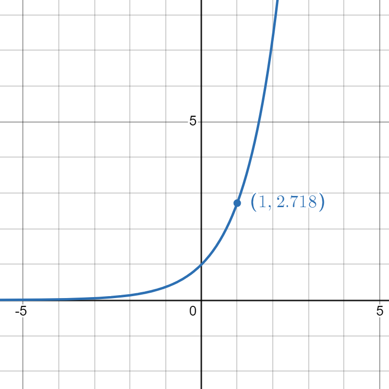
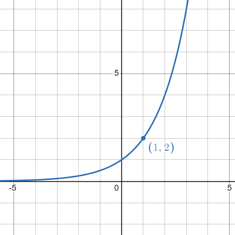
When you raise a base $a > 1$ to bigger and bigger powers, the results increase, just like the example above with $a = 8$. Let's see some graphs.

$exp1.png$

Observations:

All $ f(x) = a^x$ pass through the point $ (0,1) $, as mentioned in the fun facts.
There's no reason a base has to be a whole number! Recall the special number $e \approx 2.718 $. You can raise him to the $x$ no problem, and you can see that his (red) graph lies between $f(x) = 2^x$ and $g(x) = 3^x$, just as $ 2< 2.718 < 3 $.
On the left side of the graph, as $x \rightarrow -\infty$, the graphs hug a horizontal asymptote $ y = 0$. This makes sense because plugging in negative numbers as powers produces smaller and smaller numbers. For example,
\[ 2^{-1} = \frac{1}{2}, \quad 2^{-2} = \frac{1}{4}, \quad 2^{-5} = \frac{1}{32}, \quad ... \notag \]
These functions are always positive! (They're always above the $x$-axis.)
Since $a^1 = a $ for any $a$, you can see that they each pass through the point $ (1,a)$ matching their base. For example, $f(x) = 2^x$ passes through $ (1,2)$.
Looking out at end behavior as $x \rightarrow \infty$, the bigger the base, the steeper the function (the faster it grows).

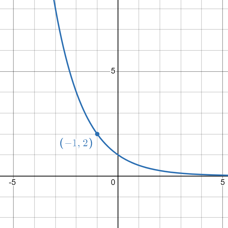
On the other hand, if $0< a < 1$, raising to higher and higher powers causes the function value to decrease. Consider $a = \frac{1}{2} $...

\[ \left( \frac{1}{2} \right)^{-1} = 2, \quad \quad \left( \frac{1}{2} \right)^0 = 1, \quad \quad \left( \frac{1}{2} \right)^1 = \frac{1}{2} , \quad \quad \left( \frac{1}{2} \right)^2 = \frac{1}{4}, \quad ... \notag \]

$exp2.png$

Observations (reason through them as above):

The graphs all still pass through $ (0,1) $.
The graphs hug a horizontal asymptote $ y = 0$ as $x \rightarrow \infty$.
The functions are still always positive (above the $x$-axis).
The functions still pass through the point $ (1,a)$ where $a$ is their base.
The functions also pass through the point $ \left( -1, \frac{1}{a} \right) $, which is sometimes easier to pinpoint.

There's one more thing I want to call out, which I've hinted at in the graph above, labeling $h(x) = e^{-x} = \frac{1}{e}^x $. Remember your power rules! There is a relationship between the functions $f(x) = a^x$ and $ g(x)= \left( \frac{1}{a}\right)^x $.

\[ g(x) = \left( \frac{1}{a}\right)^x = \frac{1}{a^x} = a^{-x} \notag \]

You can transform $f$ into $g$ by replacing the input $x$ with $-x$, which we recall from function transformations causes a reflection about the $y$-axis. Observe below.

$exp3.png$

Test your understanding with the exercises below, and then we'll get into working with these functions.

Exercise $\PageIndex{1}$

Answer True/False:

The function $ f(x) = x^7$ is exponential with base 7.
The function $ f(x) = 7^x $ is exponential with base 7.
The function $ f(x) = 4^x$ is a horizontal reflection across the $y$-axis of the function $ g(x) = 4^{-x} $.
The function $ f(x) = 4^x$ is a horizontal reflection across the $y$-axis of the function $ g(x) = \left( \frac{1}{4} \right)^x $.
The graph of $f(x) = (1.5)^x$ is increasing.
The graph of $ f(x) = (0.25)^x$ is decreasing.
The graph of $ f(x) = 3^x $ is decreasing.
As $x \rightarrow \infty$, the graph of $ f(x) = 2^x $ is steeper (faster growing) than the graph of $ g(x) = 3^x $.
As $x \rightarrow \infty$, the graph of $ f(x) = 5^x $ is steeper (faster growing) than the graph of $g(x) = e^x $.
The graph of $ f(x) = 6^x$ passes through $ (1,6) $.
The graph of $f(x) = 3^x $ passes through $ (3,1)$.
The graph of $f(x) = a^x$ passes through $ (0,1)$ for any base $a$.
The graph of $f(x) = a^x$ passes through $ (1,0)$ for any base $a$.
There exists a value of $x$ such that $ a^x < 0 $ for any base $a$.

Answer

False. That's a polynomial (monomial) with degree 7.
True.
True.
True, this is equivalent to the previous statement.
True, the base is bigger than 1.
True, the base is smaller than 1.
False.
False, the bigger the base, the faster the growth.
True, 5 is a bigger base than $e \approx 2.71...$.
True, $f(1) = 6 $.
False, it passes through $ (1,3) $ though. At $x = 3$, $f(3) = 9$.
True, $a^0 = 1$ for any $a$.
False, $a^1 \neq 0$.
False, the function $f(x) = a^x$ is always positive.

Exercise $\PageIndex{2}$

Match the exponential functions with their graphs.

$match3.png$	$match1.png$	$match2.png$	$match4.png$
1.	2.	3.	4.
$ f(x) = e^x$	$ g(x) = 2^x $	$ h(x) = \left(\frac{1}{2}\right)^x $	$ p(x) = e^{-x} $

Answer

$h$
$f$
$ g$
$ p$

Using Exponential Functions

These functions appear all the time in real-world problems. Check out the examples below, then try the exercises section!

Example $\PageIndex{1}$

Billybob Joe borrows $100 from Marybeth Sue and she charges him 10% interest, compounded annually. That is, after one year, he owes her $ 100(1+0.1) = 110 $. (Review working with percents if you need to.) After two years, he's charged another 10% of interest on that new amount, so he owes $ 110(1+0.1) = 121 $. But wait... Notice that we could have computed $ 100(1+0.1)(1+0.1) = 100(1+0.1)^2 $ to find the amount owed after two years! Do you see the pattern?

The amount owed after $t$ years is given by an exponential function $A(t) = A_0 (1+i)^t $, where $A_0 = 100$ is the initial amount, and $i = 0.1$ is the interest rate written as a decimal. Use this function (and a calculator) to find the amount Billybob Joe owes after

3 years
5 years
10 years

If he can talk Marybeth Sue down to 7% interest, what will the new function be? Use it to find the amount he would owe at the same times, using the new interest rate.

Solution

Simply plug in the values for $t$, rounding to two decimal places because this is money:

$ A(3) = 100(1.1)^3 = 133.10 $
$ A(5) = 100(1.1)^5 = 161.05 $
$ A(10) = 100(1.1)^{10} = 259.37 $

If the interest rate changes to 7%, we just change $i$ to $0.07$ and keep everything else the same. The new function is $A(t) = 100(1.07)^t $, and the new amounts owed would be

$ A(3) = 100(1.07)^3 = 122.50$
$ A(5) = 140.26 $
$ A(10) = 196.72 $

Example $\PageIndex{2}$

I have a Petri dish containing 200 bacteria at the moment, but the count is doubling every half hour. Construct an exponential function $N(t)$ that will give the number of bacteria after $t$ hours. Use it and a calculator to find the number of bacteria after

1 hour
2 hours
5 hours

Solution

Let's reason through this like we did for interest... If we're doubling every half hour, then after 0.5 hr, I have $200(2) = 400 $. After another half hour, I have $400(2) = 200(2)(2) = 200(2)^2 = 800 $. If $h$ is the number of half-hours that have passed, I have $ 200(2)^h$ bacteria. How can I translate this to a function that takes an input of $t$ in hours? Well, if 1 hour has passed, that's 2 half-hours, so two doublings. If 2 hours have passed, then 4 half-hours have passed, that's four doublings. I just need to raise $2$ to the power $2t$ to have this effect! My function is $N(t) = 200(2)^{2t} $. I plug in the desired $t$ values:

$ N(1) = 200(2)^{2} = 800 $
$ N(2) = 200(2)^4 = 3200 $
$ N(5) = 200(2)^{10} = 204,800 $

\(x\)-value	0	1	2	3	4
\(f(x)\)	\(8^0 = 1\)	\(8^1 = 8\)	\(8^2 = 64\)	\(8^3 = 512 \)	\(8^4 = 4096\)

Search

Text Color

Text Size

Margin Size

Font Type

Example \(\PageIndex{1}\)

Solution

Example \(\PageIndex{2}\)

Solution

Learning Objectives

Exponential Functions

Exercise \(\PageIndex{1}\)

Exercise \(\PageIndex{2}\)

Using Exponential Functions

Example \(\PageIndex{1}\)

Solution

Example \(\PageIndex{2}\)

Solution