Mathematics LibreTexts

3.8: Derivatives of Inverse Functions and Logarithms

  • Page ID
    8232
  • \( \newcommand{\vecs}[1]{\overset { \scriptstyle \rightharpoonup} {\mathbf{#1}} } \)

    \( \newcommand{\vecd}[1]{\overset{-\!-\!\rightharpoonup}{\vphantom{a}\smash {#1}}} \)

    \( \newcommand{\id}{\mathrm{id}}\) \( \newcommand{\Span}{\mathrm{span}}\)

    ( \newcommand{\kernel}{\mathrm{null}\,}\) \( \newcommand{\range}{\mathrm{range}\,}\)

    \( \newcommand{\RealPart}{\mathrm{Re}}\) \( \newcommand{\ImaginaryPart}{\mathrm{Im}}\)

    \( \newcommand{\Argument}{\mathrm{Arg}}\) \( \newcommand{\norm}[1]{\| #1 \|}\)

    \( \newcommand{\inner}[2]{\langle #1, #2 \rangle}\)

    \( \newcommand{\Span}{\mathrm{span}}\)

    \( \newcommand{\id}{\mathrm{id}}\)

    \( \newcommand{\Span}{\mathrm{span}}\)

    \( \newcommand{\kernel}{\mathrm{null}\,}\)

    \( \newcommand{\range}{\mathrm{range}\,}\)

    \( \newcommand{\RealPart}{\mathrm{Re}}\)

    \( \newcommand{\ImaginaryPart}{\mathrm{Im}}\)

    \( \newcommand{\Argument}{\mathrm{Arg}}\)

    \( \newcommand{\norm}[1]{\| #1 \|}\)

    \( \newcommand{\inner}[2]{\langle #1, #2 \rangle}\)

    \( \newcommand{\Span}{\mathrm{span}}\) \( \newcommand{\AA}{\unicode[.8,0]{x212B}}\)

    \( \newcommand{\vectorA}[1]{\vec{#1}}      % arrow\)

    \( \newcommand{\vectorAt}[1]{\vec{\text{#1}}}      % arrow\)

    \( \newcommand{\vectorB}[1]{\overset { \scriptstyle \rightharpoonup} {\mathbf{#1}} } \)

    \( \newcommand{\vectorC}[1]{\textbf{#1}} \)

    \( \newcommand{\vectorD}[1]{\overrightarrow{#1}} \)

    \( \newcommand{\vectorDt}[1]{\overrightarrow{\text{#1}}} \)

    \( \newcommand{\vectE}[1]{\overset{-\!-\!\rightharpoonup}{\vphantom{a}\smash{\mathbf {#1}}}} \)

    \( \newcommand{\vecs}[1]{\overset { \scriptstyle \rightharpoonup} {\mathbf{#1}} } \)

    \( \newcommand{\vecd}[1]{\overset{-\!-\!\rightharpoonup}{\vphantom{a}\smash {#1}}} \)

    \(\newcommand{\avec}{\mathbf a}\) \(\newcommand{\bvec}{\mathbf b}\) \(\newcommand{\cvec}{\mathbf c}\) \(\newcommand{\dvec}{\mathbf d}\) \(\newcommand{\dtil}{\widetilde{\mathbf d}}\) \(\newcommand{\evec}{\mathbf e}\) \(\newcommand{\fvec}{\mathbf f}\) \(\newcommand{\nvec}{\mathbf n}\) \(\newcommand{\pvec}{\mathbf p}\) \(\newcommand{\qvec}{\mathbf q}\) \(\newcommand{\svec}{\mathbf s}\) \(\newcommand{\tvec}{\mathbf t}\) \(\newcommand{\uvec}{\mathbf u}\) \(\newcommand{\vvec}{\mathbf v}\) \(\newcommand{\wvec}{\mathbf w}\) \(\newcommand{\xvec}{\mathbf x}\) \(\newcommand{\yvec}{\mathbf y}\) \(\newcommand{\zvec}{\mathbf z}\) \(\newcommand{\rvec}{\mathbf r}\) \(\newcommand{\mvec}{\mathbf m}\) \(\newcommand{\zerovec}{\mathbf 0}\) \(\newcommand{\onevec}{\mathbf 1}\) \(\newcommand{\real}{\mathbb R}\) \(\newcommand{\twovec}[2]{\left[\begin{array}{r}#1 \\ #2 \end{array}\right]}\) \(\newcommand{\ctwovec}[2]{\left[\begin{array}{c}#1 \\ #2 \end{array}\right]}\) \(\newcommand{\threevec}[3]{\left[\begin{array}{r}#1 \\ #2 \\ #3 \end{array}\right]}\) \(\newcommand{\cthreevec}[3]{\left[\begin{array}{c}#1 \\ #2 \\ #3 \end{array}\right]}\) \(\newcommand{\fourvec}[4]{\left[\begin{array}{r}#1 \\ #2 \\ #3 \\ #4 \end{array}\right]}\) \(\newcommand{\cfourvec}[4]{\left[\begin{array}{c}#1 \\ #2 \\ #3 \\ #4 \end{array}\right]}\) \(\newcommand{\fivevec}[5]{\left[\begin{array}{r}#1 \\ #2 \\ #3 \\ #4 \\ #5 \\ \end{array}\right]}\) \(\newcommand{\cfivevec}[5]{\left[\begin{array}{c}#1 \\ #2 \\ #3 \\ #4 \\ #5 \\ \end{array}\right]}\) \(\newcommand{\mattwo}[4]{\left[\begin{array}{rr}#1 \amp #2 \\ #3 \amp #4 \\ \end{array}\right]}\) \(\newcommand{\laspan}[1]{\text{Span}\{#1\}}\) \(\newcommand{\bcal}{\cal B}\) \(\newcommand{\ccal}{\cal C}\) \(\newcommand{\scal}{\cal S}\) \(\newcommand{\wcal}{\cal W}\) \(\newcommand{\ecal}{\cal E}\) \(\newcommand{\coords}[2]{\left\{#1\right\}_{#2}}\) \(\newcommand{\gray}[1]{\color{gray}{#1}}\) \(\newcommand{\lgray}[1]{\color{lightgray}{#1}}\) \(\newcommand{\rank}{\operatorname{rank}}\) \(\newcommand{\row}{\text{Row}}\) \(\newcommand{\col}{\text{Col}}\) \(\renewcommand{\row}{\text{Row}}\) \(\newcommand{\nul}{\text{Nul}}\) \(\newcommand{\var}{\text{Var}}\) \(\newcommand{\corr}{\text{corr}}\) \(\newcommand{\len}[1]{\left|#1\right|}\) \(\newcommand{\bbar}{\overline{\bvec}}\) \(\newcommand{\bhat}{\widehat{\bvec}}\) \(\newcommand{\bperp}{\bvec^\perp}\) \(\newcommand{\xhat}{\widehat{\xvec}}\) \(\newcommand{\vhat}{\widehat{\vvec}}\) \(\newcommand{\uhat}{\widehat{\uvec}}\) \(\newcommand{\what}{\widehat{\wvec}}\) \(\newcommand{\Sighat}{\widehat{\Sigma}}\) \(\newcommand{\lt}{<}\) \(\newcommand{\gt}{>}\) \(\newcommand{\amp}{&}\) \(\definecolor{fillinmathshade}{gray}{0.9}\)

    As with the sine, we do not know anything about derivatives that allows us to compute the derivatives of the exponential and logarithmic functions without going back to basics. Let's do a little work with the definition again:

    \[\eqalign{ {d\over dx}a^x&=\lim_{\Delta x\to 0} {a^{x+\Delta x}-a^x\over \Delta x}\cr& =\lim_{\Delta x\to 0} {a^xa^{\Delta x}-a^x\over \Delta x}\cr& =\lim_{\Delta x\to 0} a^x{a^{\Delta x}-1\over \Delta x}\cr& =a^x\lim_{\Delta x\to 0} {a^{\Delta x}-1\over \Delta x}.\cr }\]

    There are two interesting things to note here: As in the case of the sine function we are left with a limit that involves \(\Delta x\) but not \(x\), which means that whatever \( \lim_{\Delta x\to 0} (a^{\Delta x}-1)/\Delta x\) is, we know that it is a number, that is, a constant. This means that \( a^x\) has a remarkable property: its derivative is a constant times itself.

    We earlier remarked that the hardest limit we would compute is \( \lim_{x\to0}\sin x/x=1\); we now have a limit that is just a bit too hard to include here. In fact the hard part is to see that \( \lim_{\Delta x\to 0} (a^{\Delta x}-1)/\Delta x\) even exists---does this fraction really get closer and closer to some fixed value? Yes it does, but we will not prove this fact.

    We can look at some examples. Consider \( (2^x-1)/x\) for some small values of \(x\): 1, \(0.828427124\), \(0.756828460\), \(0.724061864\), \(0.70838051\), \(0.70070877\) when \(x\) is 1, \(1/2\), \(1/4\), \(1/8\), \(1/16\), \(1/32\), respectively. It looks like this is settling in around \(0.7\), which turns out to be true (but the limit is not exactly \(0.7\)). Consider next \( (3^x-1)/x\): \(2\), \(1.464101616\), \(1.264296052\), \(1.177621520\), \(1.13720773\), \(1.11768854\), at the same values of \(x\). It turns out to be true that in the limit this is about \(1.1\).

    Two examples don't establish a pattern, but if you do more examples you will find that the limit varies directly with the value of \(a\): bigger \(a\), bigger limit; smaller \(a\), smaller limit. As we can already see, some of these limits will be less than 1 and some larger than 1. Somewhere between \(a=2\) and \(a=3\) the limit will be exactly 1; the value at which this happens is called \(e\), so that

    \[\lim_{\Delta x\to 0} {e^{\Delta x}-1\over \Delta x}=1.\]

    As you might guess from our two examples, \(e\) is closer to 3 than to 2, and in fact \(e\approx 2.718\).

    Now we see that the function \( e^x\) has a truly remarkable property:

    \[\eqalign{ {d\over dx}e^x&=\lim_{\Delta x\to 0} {e^{x+\Delta x}-e^x\over \Delta x}\cr& =\lim_{\Delta x\to 0} {e^xe^{\Delta x}-e^x\over \Delta x}\cr& =\lim_{\Delta x\to 0} e^x{e^{\Delta x}-1\over \Delta x}\cr& =e^x\lim_{\Delta x\to 0} {e^{\Delta x}-1\over \Delta x}\cr& =e^x.\cr }\]

    That is, \( e^x\) is its own derivative, or in other words the slope of \( e^x\) is the same as its height, or the same as its second coordinate: The function \( f(x)=e^x\) goes through the point \( (z,e^z)\) and has slope \( e^z\) there, no matter what \(z\) is. It is sometimes convenient to express the function \( e^x\) without an exponent, since complicated exponents can be hard to read. In such cases we use \(\exp(x)\), e.g., \( \exp(1+x^2)\) instead of \( e^{1+x^2}\).

    What about the logarithm function? This too is hard, but as the cosine function was easier to do once the sine was done, so the logarithm is easier to do now that we know the derivative of the exponential function. Let's start with \( \log_e x\), which as you probably know is often abbreviated \(\ln x\) and called the "natural logarithm'' function.

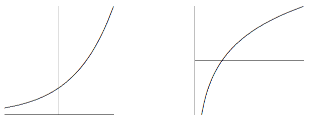
    Consider the relationship between the two functions, namely, that they are inverses, that one "undoes'' the other. Graphically this means that they have the same graph except that one is "flipped'' or "reflected'' through the line \(y=x\), as shown in Figure \(\PageIndex{1}\).

    alt

    Figure \(\PageIndex{1}\): The exponential (green) and logarithmic (blue) functions. As inverses of each other, their graphs are reflections of each other across the line \(y=x\) (dashed).

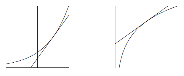
    This means that the slopes of these two functions are closely related as well: For example, the slope of \( e^x\) is \(e\) at \(x=1\); at the corresponding point on the \(\ln(x)\) curve, the slope must be \(1/e\), because the "rise'' and the "run'' have been interchanged. Since the slope of \( e^x\) is \(e\) at the point \((1,e)\), the slope of \(\ln(x)\) is \(1/e\) at the point \((e,1)\).

    alt

    Figure \(\PageIndex{2}\): The exponential (green) and logarithmic (blue) functions. The dashed lines indicate the slope of the respective functions at the points \((1,e)\) and \((e,1)\). It is interesting to note that these lines intersect at the origin.

    More generally, we know that the slope of \( e^x\) is \( e^z\) at the point \( (z,e^z)\), so the slope of \(\ln(x)\) is \( 1/e^z\) at \( (e^z,z)\), as indicated in Figure \(\PageIndex{2}\). In other words, the slope of \(\ln x\) is the reciprocal of the first coordinate at any point; this means that the slope of \(\ln x\) at \((x,\ln x)\) is \(1/x\). The upshot is: \({d\over dx}\ln x = {1\over x}.\) We have discussed this from the point of view of the graphs, which is easy to understand but is not normally considered a rigorous proof---it is too easy to be led astray by pictures that seem reasonable but that miss some hard point. It is possible to do this derivation without resorting to pictures, and indeed we will see an alternate approach soon.

    Note that \(\ln x\) is defined only for \(x>0\). It is sometimes useful to consider the function \(\ln |x|\), a function defined for \(x\not=0\). When \(x < 0\), \(\ln |x|=\ln(-x)\) and

    \[{d\over dx}\ln |x|={d\over dx}\ln (-x)={1\over -x}(-1)={1\over x}.\]

    Thus whether \(x\) is positive or negative, the derivative is the same.

    What about the functions \( a^x\) and \( \log_a x\)? We know that the derivative of \( a^x\) is some constant times \( a^x\) itself, but what constant? Remember that "the logarithm is the exponent'' and you will see that \( a=e^{\ln a}\). Then \(a^x = (e^{\ln a})^x = e^{x\ln a},\) and we can compute the derivative using the chain rule:

    \[{d\over dx} a^x = {d\over dx}(e^{\ln a})^x = {d\over dx}e^{x\ln a} = (\ln a)e^{x\ln a} =(\ln a)a^x.\]

    The constant is simply \(\ln a\). Likewise we can compute the derivative of the logarithm function \( \log_a x\). Since \(x=e^{\ln x}\) we can take the logarithm base \(a\) of both sides to get \( \log_a(x)=\log_a(e^{\ln x})=\ln x \log_a e\). Then

    \[{d\over dx}\log_a x = {1\over x}\log_a e.\]

    This is a perfectly good answer, but we can improve it slightly. Since

    \[\eqalign{ a&=e^{\ln a}\cr \log_a(a) &= \log_a(e^{\ln a}) = \ln a\log_a e\cr 1&=\ln a\log_a e\cr {1\over \ln a}&=\log_a e,\cr }\]

    we can replace \( \log_a e\) to get \({d\over dx}\log_a x = {1\over x\ln a}\).

    You may if you wish memorize the formulas

    \[{d\over dx}a^x = (\ln a)a^x \quad \hbox{and}\quad {d\over dx}\log_a x = {1\over x\ln a}.\]

    Because the "trick'' \( a=e^{\ln a}\) is often useful, and sometimes essential, it may be better to remember the trick, not the formula.

    Example \(\PageIndex{1}\)

    Compute the derivative of \( f(x)=2^x\).

    Solution

    \[\eqalign{ {d\over dx}2^{x} &= {d\over dx}(e^{\ln 2})^x\cr& = {d\over dx}e^{x\ln 2}\cr& = \left({d\over dx} x\ln 2\right) e^{x\ln 2}\cr& = (\ln 2) e^{x\ln 2}=2^x\ln2\cr }\]

    Example \(\PageIndex{2}\)

    Compute the derivative of \( f(x)=2^{x^2}=2^{(x^2)}\).

    \[\eqalign{ {d\over dx}2^{x^2} &= {d\over dx}e^{x^2\ln 2}\cr& = \left({d\over dx} x^2\ln 2\right) e^{x^2\ln 2}\cr& = (2\ln 2) x e^{x^2\ln 2}\cr& = (2\ln 2) x 2^{x^2}\cr }\]

    Example \(\PageIndex{3}\)

    Compute the derivative of \( f(x)=x^x\). At first this appears to be a new kind of function: it is not a constant power of \(x\), and it does not seem to be an exponential function, since the base is not constant. But in fact it is no harder than the previous example.

    \[\eqalign{ {d\over dx}x^x&={d\over dx}e^{x\ln x}\cr& =\left({d\over dx}x\ln x\right)e^{x\ln x}\cr& =(x{1\over x}+\ln x)x^x\cr& =(1+\ln x)x^x\cr }\]

    Example \(\PageIndex{4}\)

    Recall that we have not justified the power rule except when the exponent is a positive or negative integer. We can use the exponential function to take care of other exponents.

    \[\eqalign{ {d\over dx}x^r&={d\over dx}e^{r\ln x}\cr& =\left({d\over dx}r\ln x\right)e^{r\ln x}\cr& =(r{1\over x})x^r\cr& =rx^{r-1}\cr }\]

    Contributors

    David Guichard (Whitman College)

    • Integrated by Justin Marshall.


    3.8: Derivatives of Inverse Functions and Logarithms is shared under a CC BY-NC-SA license and was authored, remixed, and/or curated by LibreTexts.

    • Was this article helpful?