Mathematics LibreTexts

4.4: Concavity and Curve Sketching

  • Page ID
    8240
  • \( \newcommand{\vecs}[1]{\overset { \scriptstyle \rightharpoonup} {\mathbf{#1}} } \)

    \( \newcommand{\vecd}[1]{\overset{-\!-\!\rightharpoonup}{\vphantom{a}\smash {#1}}} \)

    \( \newcommand{\id}{\mathrm{id}}\) \( \newcommand{\Span}{\mathrm{span}}\)

    ( \newcommand{\kernel}{\mathrm{null}\,}\) \( \newcommand{\range}{\mathrm{range}\,}\)

    \( \newcommand{\RealPart}{\mathrm{Re}}\) \( \newcommand{\ImaginaryPart}{\mathrm{Im}}\)

    \( \newcommand{\Argument}{\mathrm{Arg}}\) \( \newcommand{\norm}[1]{\| #1 \|}\)

    \( \newcommand{\inner}[2]{\langle #1, #2 \rangle}\)

    \( \newcommand{\Span}{\mathrm{span}}\)

    \( \newcommand{\id}{\mathrm{id}}\)

    \( \newcommand{\Span}{\mathrm{span}}\)

    \( \newcommand{\kernel}{\mathrm{null}\,}\)

    \( \newcommand{\range}{\mathrm{range}\,}\)

    \( \newcommand{\RealPart}{\mathrm{Re}}\)

    \( \newcommand{\ImaginaryPart}{\mathrm{Im}}\)

    \( \newcommand{\Argument}{\mathrm{Arg}}\)

    \( \newcommand{\norm}[1]{\| #1 \|}\)

    \( \newcommand{\inner}[2]{\langle #1, #2 \rangle}\)

    \( \newcommand{\Span}{\mathrm{span}}\) \( \newcommand{\AA}{\unicode[.8,0]{x212B}}\)

    \( \newcommand{\vectorA}[1]{\vec{#1}}      % arrow\)

    \( \newcommand{\vectorAt}[1]{\vec{\text{#1}}}      % arrow\)

    \( \newcommand{\vectorB}[1]{\overset { \scriptstyle \rightharpoonup} {\mathbf{#1}} } \)

    \( \newcommand{\vectorC}[1]{\textbf{#1}} \)

    \( \newcommand{\vectorD}[1]{\overrightarrow{#1}} \)

    \( \newcommand{\vectorDt}[1]{\overrightarrow{\text{#1}}} \)

    \( \newcommand{\vectE}[1]{\overset{-\!-\!\rightharpoonup}{\vphantom{a}\smash{\mathbf {#1}}}} \)

    \( \newcommand{\vecs}[1]{\overset { \scriptstyle \rightharpoonup} {\mathbf{#1}} } \)

    \( \newcommand{\vecd}[1]{\overset{-\!-\!\rightharpoonup}{\vphantom{a}\smash {#1}}} \)

    \(\newcommand{\avec}{\mathbf a}\) \(\newcommand{\bvec}{\mathbf b}\) \(\newcommand{\cvec}{\mathbf c}\) \(\newcommand{\dvec}{\mathbf d}\) \(\newcommand{\dtil}{\widetilde{\mathbf d}}\) \(\newcommand{\evec}{\mathbf e}\) \(\newcommand{\fvec}{\mathbf f}\) \(\newcommand{\nvec}{\mathbf n}\) \(\newcommand{\pvec}{\mathbf p}\) \(\newcommand{\qvec}{\mathbf q}\) \(\newcommand{\svec}{\mathbf s}\) \(\newcommand{\tvec}{\mathbf t}\) \(\newcommand{\uvec}{\mathbf u}\) \(\newcommand{\vvec}{\mathbf v}\) \(\newcommand{\wvec}{\mathbf w}\) \(\newcommand{\xvec}{\mathbf x}\) \(\newcommand{\yvec}{\mathbf y}\) \(\newcommand{\zvec}{\mathbf z}\) \(\newcommand{\rvec}{\mathbf r}\) \(\newcommand{\mvec}{\mathbf m}\) \(\newcommand{\zerovec}{\mathbf 0}\) \(\newcommand{\onevec}{\mathbf 1}\) \(\newcommand{\real}{\mathbb R}\) \(\newcommand{\twovec}[2]{\left[\begin{array}{r}#1 \\ #2 \end{array}\right]}\) \(\newcommand{\ctwovec}[2]{\left[\begin{array}{c}#1 \\ #2 \end{array}\right]}\) \(\newcommand{\threevec}[3]{\left[\begin{array}{r}#1 \\ #2 \\ #3 \end{array}\right]}\) \(\newcommand{\cthreevec}[3]{\left[\begin{array}{c}#1 \\ #2 \\ #3 \end{array}\right]}\) \(\newcommand{\fourvec}[4]{\left[\begin{array}{r}#1 \\ #2 \\ #3 \\ #4 \end{array}\right]}\) \(\newcommand{\cfourvec}[4]{\left[\begin{array}{c}#1 \\ #2 \\ #3 \\ #4 \end{array}\right]}\) \(\newcommand{\fivevec}[5]{\left[\begin{array}{r}#1 \\ #2 \\ #3 \\ #4 \\ #5 \\ \end{array}\right]}\) \(\newcommand{\cfivevec}[5]{\left[\begin{array}{c}#1 \\ #2 \\ #3 \\ #4 \\ #5 \\ \end{array}\right]}\) \(\newcommand{\mattwo}[4]{\left[\begin{array}{rr}#1 \amp #2 \\ #3 \amp #4 \\ \end{array}\right]}\) \(\newcommand{\laspan}[1]{\text{Span}\{#1\}}\) \(\newcommand{\bcal}{\cal B}\) \(\newcommand{\ccal}{\cal C}\) \(\newcommand{\scal}{\cal S}\) \(\newcommand{\wcal}{\cal W}\) \(\newcommand{\ecal}{\cal E}\) \(\newcommand{\coords}[2]{\left\{#1\right\}_{#2}}\) \(\newcommand{\gray}[1]{\color{gray}{#1}}\) \(\newcommand{\lgray}[1]{\color{lightgray}{#1}}\) \(\newcommand{\rank}{\operatorname{rank}}\) \(\newcommand{\row}{\text{Row}}\) \(\newcommand{\col}{\text{Col}}\) \(\renewcommand{\row}{\text{Row}}\) \(\newcommand{\nul}{\text{Nul}}\) \(\newcommand{\var}{\text{Var}}\) \(\newcommand{\corr}{\text{corr}}\) \(\newcommand{\len}[1]{\left|#1\right|}\) \(\newcommand{\bbar}{\overline{\bvec}}\) \(\newcommand{\bhat}{\widehat{\bvec}}\) \(\newcommand{\bperp}{\bvec^\perp}\) \(\newcommand{\xhat}{\widehat{\xvec}}\) \(\newcommand{\vhat}{\widehat{\vvec}}\) \(\newcommand{\uhat}{\widehat{\uvec}}\) \(\newcommand{\what}{\widehat{\wvec}}\) \(\newcommand{\Sighat}{\widehat{\Sigma}}\) \(\newcommand{\lt}{<}\) \(\newcommand{\gt}{>}\) \(\newcommand{\amp}{&}\) \(\definecolor{fillinmathshade}{gray}{0.9}\)

    We know that the sign of the derivative tells us whether a function is increasing or decreasing; for example, when \(f'(x)>0\), \(f(x)\) is increasing. The sign of the second derivative \(f''(x)\) tells us whether \(f'\) is increasing or decreasing; we have seen that if \(f'\) is zero and increasing at a point then there is a local minimum at the point, and if \(f'\) is zero and decreasing at a point then there is a local maximum at the point. Thus, we extracted information about \(f\) from information about \(f''\).

    We can get information from the sign of \(f''\) even when \(f'\) is not zero. Suppose that \(f''(a)>0\). This means that near \(x=a\), \(f'\) is increasing. If \(f'(a)>0\), this means that \(f\) slopes up and is getting steeper; if \(f'(a) < 0\), this means that \(f\) slopes down and is getting less steep. The two situations are shown in Figure \(\PageIndex{1}\). A curve that is shaped like this is called concave up.

    f''(a)>0: f'(a) positive and increasing, f'(a) negative and increasing

    Figure \(\PageIndex{1}\): \(f''(a)>0\): \(f'(a)\) positive and increasing, \(f'(a)\) negative and increasing.

    Now suppose that \(f''(a) < 0\). This means that near \(x=a\), \(f'\) is decreasing. If \(f'(a)>0\), this means that \(f\) slopes up and is getting less steep; if \(f'(a) < 0\), this means that \(f\) slopes down and is getting steeper. The two situations are shown in Figure \(\PageIndex{2}\). A curve that is shaped like this is called concave down.
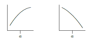
    f''(a) < 0: f'(a) positive and decreasing, f'(a) negative and decreasing.

    Figure \(\PageIndex{2}\): \(f''(a) < 0\): \(f'(a)\) positive and decreasing, \(f'(a)\) negative and decreasing.

    If we are trying to understand the shape of the graph of a function, knowing where it is concave up and concave down helps us to get a more accurate picture. Of particular interest are points at which the concavity changes from up to down or down to up; such points are called inflection points. If the concavity changes from up to down at \(x=a\), \(f''\) changes from positive to the left of \(a\) to negative to the right of \(a\), and usually \(f''(a)=0\). We can identify such points by first finding where \(f''(x)\) is zero and then checking to see whether \(f''(x)\) does in fact go from positive to negative or negative to positive at these points. Note that it is possible that \(f''(a)=0\) but the concavity is the same on both sides; \( f(x)=x^4\) at \(x=0\) is an example.

    Example \(\PageIndex{1}\)

    Describe the concavity of \( f(x)=x^3-x\).

    Solution

    The first dervative is \( f'(x)=3x^2-1\) and the second is \(f''(x)=6x\).

    Since \(f''(0)=0\), there is potentially an inflection point at zero. Since \(f''(x)>0\) when \(x>0\) and \(f''(x) < 0\) when \(x < 0\) the concavity does change from down to up at zero, and the curve is concave down for all \(x < 0\) and concave up for all \(x>0\).

    Note that we need to compute and analyze the second derivative to understand concavity, so we may as well try to use the second derivative test for maxima and minima. If for some reason this fails we can then try one of the other tests.

    Contributors

    David Guichard (Whitman College)

    • Integrated by Justin Marshall.


    4.4: Concavity and Curve Sketching is shared under a CC BY-NC-SA license and was authored, remixed, and/or curated by LibreTexts.

    • Was this article helpful?