15.1: Double and Iterated Integrals over Rectangles

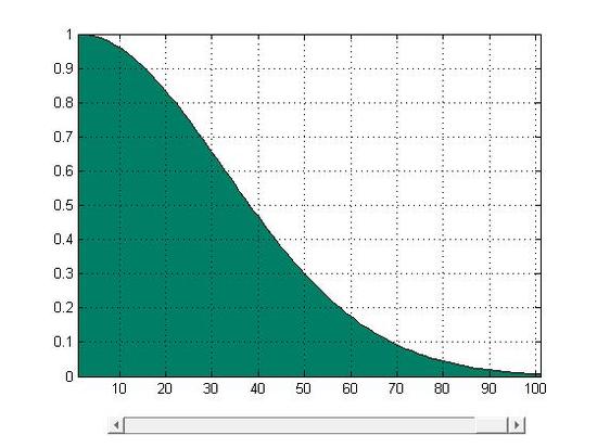
$$y=f(x)=e^{-5x^2} , 0\leq x \leq 1 \nonumber$$

Figure 15.1-0

$$\int_a^b f(x)\;dx = \lim_{n\rightarrow\infty}\sum_{i=1}^n f(x_i)\, \Delta x_i \nonumber$$

A fundamental method to calculate the area: the base of function f(x) is equally divide into n pieces whose width are $\Delta x$. Then $S=\Delta x f(x_i)$ is the area of the rectangle at the location $\Delta x_i$ and its height is $f(x_i)$ among the range $\Delta x_i$. Through summing all these rectangular pieces together, we can roughly estimate the area under the function $f(x)$ in its domain. The equation $\sum_{i=1}^n f(x_i)\, \Delta x_i$ can be used to represent this process.

However, $\sum_{i=1}^n f(x_i)\, \Delta x_i$ can only help us to estimate the value, which means errors still exist. In this case, limits help us to fix the problem.

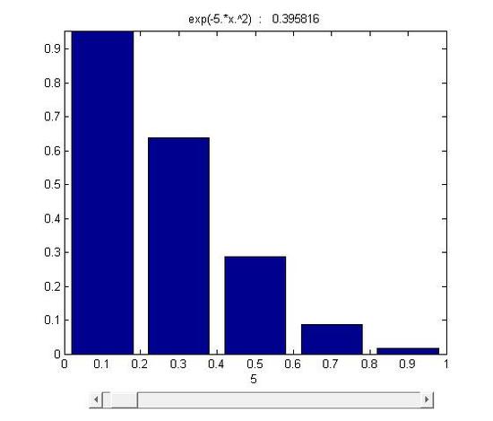
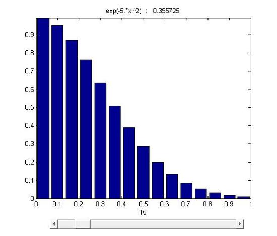
figure 15.1-1

As it was mentioned, the area was divided into n stripes. As $n \rightarrow \infty$ and $\Delta x \rightarrow 0$, stripes$\Delta x f(x_i)$approachs to a line whose length is equal to the height of $f(x_i)$. Eventually, through infinite division and accumulation, the error is reduced to zero and the sum of $f(x) \Delta x$ equals to the area under the curve.

$$\int_a^b f(x)\;dx = \lim_{n\rightarrow\infty}\sum_{i=1}^n f(x_i)\, \Delta x_i \nonumber$$

Thus, we can conclude that the integral is the function of accumulation as it accumulates infinite number of strips in a certain domain to calculate the area. Similarly, the double integral is also a function of accumulation. It accumulates infinite number of small 3D strips to calculate the volume of 3D objects.

$$V=\int \int_R f(x_i,y_i) dx= \lim_{n\rightarrow\infty}\sum_{k=1}^n f(x_i,y_i)\Delta A_i \nonumber$$

$R$ is the domain of the function (the area that you want to integrate over)

Explanation:as $n \rightarrow \infty$, the number of strips goes to infinity, $\Delta A \rightarrow\infty$, the error of calculation goes to 0 and the accumulation of these infinite strips eventually equals the volume of the objects.

Theoretical discussion with descriptive elaboration

Theorem: Fubini's Theorem (First Form)

If $f(x,y)$ is contunuous throughout the rectangular region R: $a\leq x \leq b, c\leq y \leq d,$

then

$$\int \int_R f(x,y)\Delta A=\int_c^d \int_a^b f(x,y)\Delta x \Delta y= \int_a^b \int_c^d f(x,y)\Delta y \Delta x. \nonumber$$

Fubini's Theorem is usually used to calculate the volume of three dimensional bodies

Figure 15.1-2

$$V_i= f(x_i,y_i) \Delta A_i= f(x_i,y_i)\Delta x \Delta y \nonumber$$

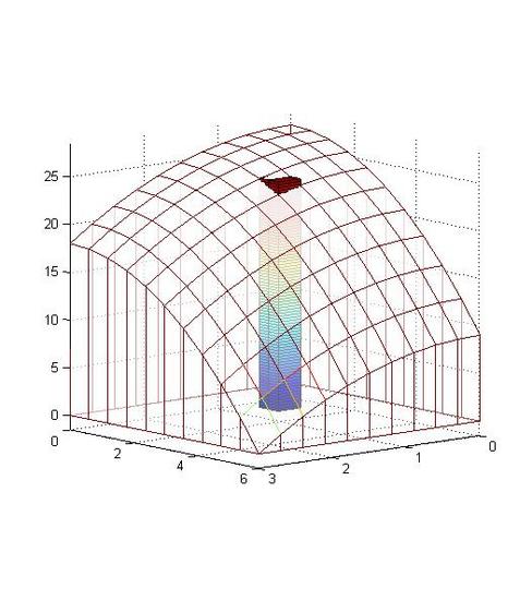
In figure 15.1-2 , $f(x_i,y_i)$ is the height of the cuboid and $\Delta A$ is its base. $V_i$ means that at different location, there is a corresponding cuboid whose height is closed to the average height of the graph at the area $\Delta A_i$.

Figure 15.1-3

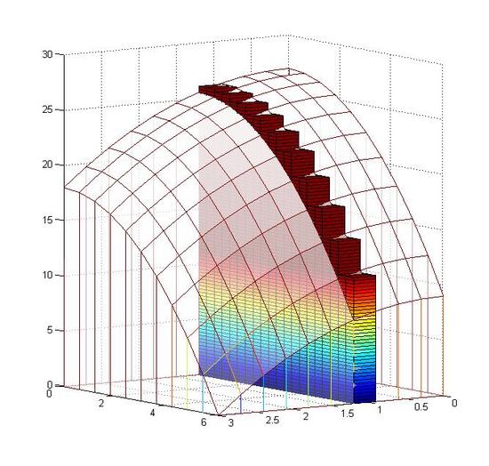
At the specific $\Delta y_i$, the cuboids with different $\Delta x_i$ are lined up to form a layer.

Figure 15.1-4

$$V= \sum_{i=1}^n f(x_i,y_i) \, \Delta A_i=\sum_{i=1}^n f(x_i,y_i)\Delta x_i \Delta y_i \nonumber$$

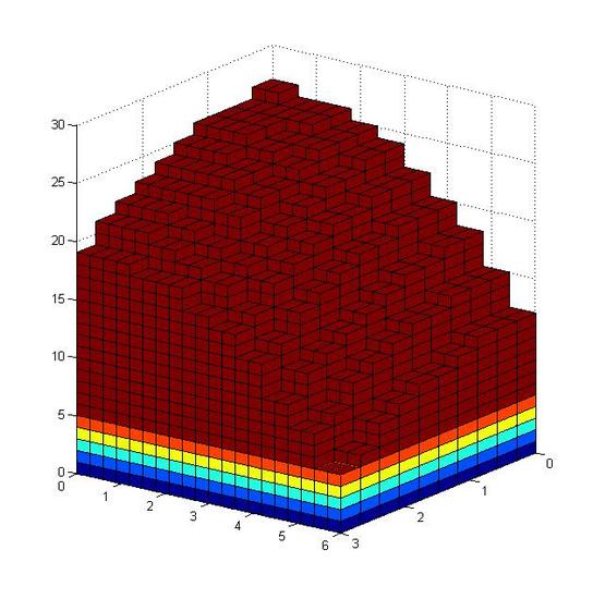
As all the layers are combined together, we get a body that is approximated to the one in the next graph, but the error is still very large.

Figure 15.1-5

$$V=\lim_{n\rightarrow \infty } \sum_{i=1}^n f(x_i,y_i) \, \Delta A_i \nonumber$$

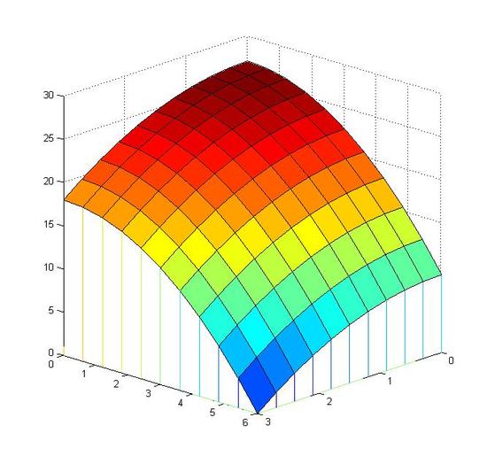
Limit helps to solve this problem. As n goes to infinity, $\Delta A_i$ becomes smaller eventually turns to a dot. $f(x_i, y_i) \Delta A_i$ becomes a line and error of volume decreases to zero. Thus, the accumulation of all these lines equal to the volume.

Example 1

Now we can calculate the volume below the function $f(x,y)=27-x^2-\frac{1}{2}y^2dx dy$ and above $f(x,y)$, in the domain $0\leq x \leq 3$ and $0 \leq y \leq 6$.

$$\begin{align} & \int_0^6 \int_0^3 27-x^2-\frac{1}{2} y^2dx dy \\ & =\int_0^6 (27-\frac{1}{2}y^2)x-\frac{1}{3}x^3 \Big|_0^3 dy \\ & =\int_0^6 [(27-\frac{1}{2}y^2)\times3-\frac{1}{3}\times 3^3 \\ & =\int_0^6 72-\frac{3}{2}y^2 \ dy \\ & =[72y-\frac{1}{2}y^3]\Big|_0^6 \\ & = (72\times 6-\frac{1}{2}\times6^3)-(0-0) \\ & = 324 \end{align} \nonumber$$

Figure: (left) from step 1 to step 3 (right) from step 3 to step 6

Example 2

Another way to calculate the volume of the graph:

$$\begin{align} &\int_0^3 \int_0^6 27-x^2-\frac{1}{2} y^2dy dx \\ & = \int_0^3 (27-x^2)y-\frac{1}{6}y^3 \Big|_0^6 \ dx \\ & =\int_0^3 [(27-x^2)\times 6 -\frac{1}{6}\times6^3]-[0-0]\ dx \\ & =\int_0^3 126-6x^2\ dx \\ & = [126x-2x^3]\Big|_0^3 \\ & = (126\times3-2\times 3^3 )-(0-0) \\ & = 324. \end{align} \nonumber$$

Reminder: the positions of $\Delta x$ and $\Delta y$ are different. So are the positions of their domains.

Example 3

Find the volume that is bounded above by the surface $z=f(x,y)=x^2+y^2$ and below by a rectangule R: $0\leq x \leq 2, 0\leq y \leq 3$.

$$\begin{align} & \int_0^2 \int_0^3 x^2+y^2 dy dx \\ & =\int_0^2 x^2y+\frac{1}{3}y^3 \Big|_0^3 dx \\ & =\int_0^2 3x^2+9 dx \\ & =x^3+9x\Big|_0^2 \\ & =(8+18)-0 \\ & =26 \end{align} \nonumber$$

Contributors and Attributions

Integrated by Justin Marshall.