3.2: Linear Functions

In this section, we will focus on a particular type of function known as a linear function. Much can be said about linear functions, and in fact there is an entire branch of mathematics, linear algebra, devoted to the study of linear functions! We will focus more on the applications of linear functions in this chapter.

In this section, you will learn to:

• Recognize examples and non-examples of linear functions
• Use linear functions to model real-world situations
• Describe various geometric properties of linear functions, including their slope

Linear Functions

Instead of starting this section with a definition, as usual, we will start with an example.

Example \(\PageIndex{1}\)

For most residential customers who are connected to city water, the city of Monmouth charges a basic monthly water use \(\$22.48\) fee each month, plus a \(\$.0323\) per cubic foot of water used. Write a function that describes the cost of a monthly water bill in Monmouth in terms of the number of cubic feet of water used. (Note: these numbers are accurate as of 2023.)

Solution

Before we start trying to write a function, let's think about a few examples. If you used \(100\) cubic feet of water (a very small amount for monthly water use), you would have to pay \(100 \times \$0.0323 = \$3.23\) for that 100 cubic feet of water, plus the basic fee charge. So the total would be calculated as follows:

\[\left(\underset{\text{rate per cubic foot } \times \text{ cubic feet }} {\$0.0323 \times 100}\right) + \underset{\text{ basic fee }}{\$22.48} = \$25.71\]

That is not too bad, since we are using exactly 100 cubic feet. What if you use 200 cubic feet? Well, in that case, we have to pay the volume rate twice. In that case, we would have:

\[\left(\underset{\text{rate per cubic foot } \times \text{ cubic feet }} {\$0.0323 \times 200}\right) + \underset{\text{ basic fee }}{\$22.48} = \$28.94\]

That is, we are taking the number of cubic feet of water, multiplying it by the rate per cubic foot, and then adding the basic fee. Either way, the basic fee does not change from month to month, but the amount you pay for water does -- it is determined by your usage.

So, for a general formula, we could use \(w\) to stand for the number of cubic feet of water used, and \(C(w)\) to stand for the cost of the water bill in dollars. Remember: this is function notation, and it simply means that the cost is dependent upon the amount of water used. It is not denoting multiplication!

Therefore, a function that represents this situation is: \[C(w) = 0.0323 w + 22.48\]

That may not have been obvious, but now that you've seen it, perhaps you can recognize similar situations in the future. There are two components to this situation: a flat fee, and a per unit rate. The per unit rate is multiplied by the number of units used. In the previous example, the units were cubic feet, and the per unit rate was \(\$0.0323\) per cubic foot of water. The basic fee, or flat fee, is a cost that does not change based on usage, and is just added onto the bill. In the previous example, the flat fee was \(\$22.48\). There are many things that are charged this way. We will see some examples, and if you think about bills you or your family pay, you can likely think of more.

This common function structure, which shows up not only in bills but in many other places, has a special name.

Definition: Linear Functions

A linear function is a function that can be written \(f(x) = mx + b\) for some numbers \(m\) and \(b\). The number \(m\) is called the slope of the function, and represents the rate of change of the function. The number \(b\) is called the vertical intercept of the function, and represents the starting value of the function. The graph of a linear function looks like a straight line.

Let's see a couple examples.

Example \(\PageIndex{2}\)

Is the water bill example from the previous problem a linear function? If so, find its slope and vertical intercept and interpret them in the context of the question. Evaluate \(C(500)\), graph the corresponding point, and explain its significance.

Solution

The formula from the previous problem is indeed a linear function. Recall, we found that:  \[C(w) =0.0323w + 22.48 \]

where \(w\) was the number of cubic feet of water used and \(C(w)\) was the cost associated to that usage. We see that indeed, this has the form \(mx+ b\), where \(m = 0.0323\) and \(b = 22.48\). You may notice that instead of the variable \(x\) and function name \(f\), the function \(C(w)\) uses a \(C\) and a \(w\) instead. This is intentional, and shows that the letter names for the variable and function don't affect whether the function is linear. We are free to choose letters as we see fit to match the context of the problem. In this problem, \(w\) stood for the amount of water, and \(C\) stood for the cost of the bill, which will help us remember their meaning when we need to interpret our answer later.

Since we know \(C(w) =0.0323w + 22.48\) is linear, we can see that its slope is \(0.0323\), and its vertical intercept is \(22.48\). In context, the slope represents the fact that each cubic foot of water costs \(\$0.0323\) that is, it is the rate of change of the cost with respect to usage. The vertical intercept in this case is \(22.48\), which represents the flat fee, or starting value. In other words, it is the amount you would pay if you used no water at all.

To graph this, we can use the methods we learned in the previous section: either we can make a table of values, or we can use graphing software (such as Desmos). Desmos produces this picture:

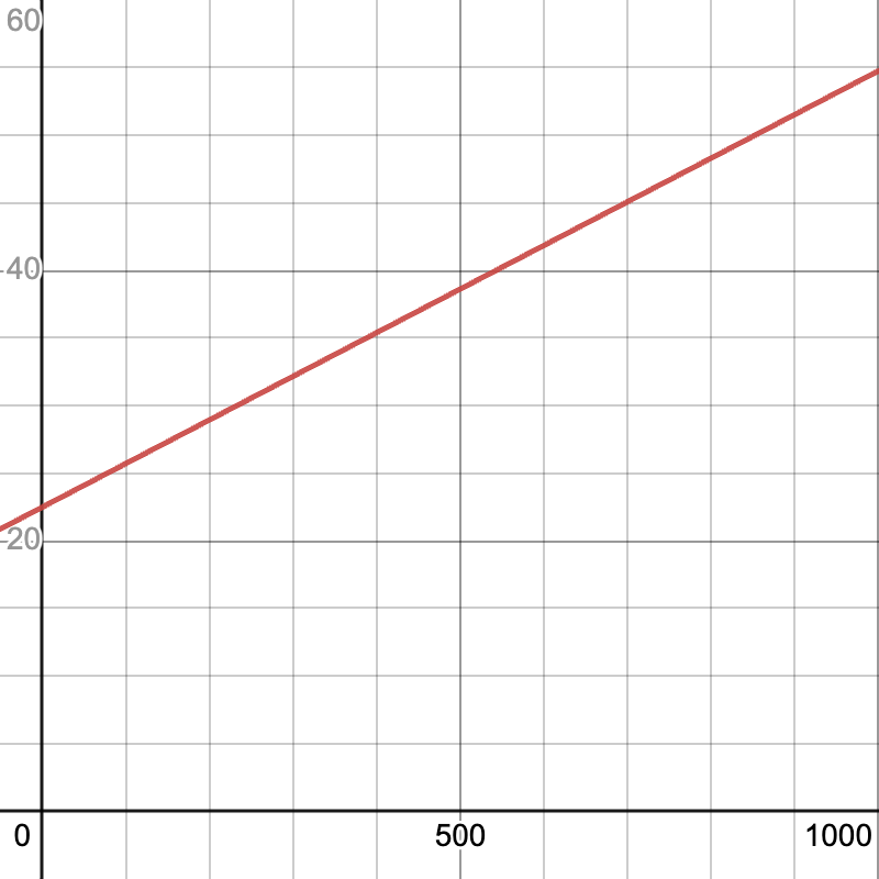
On this picture, we see that the line crosses the vertical axis just above the \(20\) line. The exact spot it is crossing is at \(22.48\), which is the vertical intercept of the function. That shows the flat fee that is paid when \(0\) cubic feet of water are used.

As we move to the right, the horizontal axis shows how many cubic feet of water are used. As that number increases, the value of the function (which is the vertical value of the red line) increases. For example, when the number of cubic feet of water used is \(500\), we can look at \(500\) on the horizontal axis. The value of the function at that point, which is between \(35\) and \(40\) on the vertical axis, is the cost associated with \(500\) cubic feet of water usage. We can calculate the exact value of this point by computing: \[C(500) = 0.0323 \times 500 + 22.48 = 38.63\]

That is, if you use \(500\) cubic feet of water, your water bill will be \(\$38.63\). The graph gives us an easy way to estimate any the cost associated with any number of cubic feet. The formula allows us to calculate exact values.

Here is the graph again, this time with the relevant points labeled.

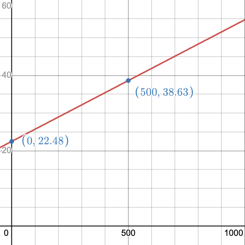
Take a look at the calculations again, and make sure that you understand how they relate to the graph. The first coordinate of each ordered pair corresponds to the amount of water used, and the second coordinate corresponds to the cost of the bill. The graph gives us a way to visualize the entire relationship between water used and cost.

Properties of Linear Functions

Something you may have noticed about the water bill example is that the cost went up at a constant rate when compared to the water usage. This is the hallmark of linear functions -- a constant rate of change. This constant rate of change can either be increasing or decreasing. If it is an increasing linear function, the same amount will be added to the output for every increase of one in the input. If it is a decreasing linear function, the same amount will be subtracted from the output for each increase in the input.

Example \(\PageIndex{3}\)

Each of the following tables represents a function. Which one(s) could be linear? Explain why you know.

1. \(x\)	\(f(x)\)
   1	2
   2	4
   3	8
   4	16

2. \(x\)	\(g(x)\)
   1	4
   2	1
   3	-2
   4	-5

Solution

Let's look at the table a, which describes a function, \(f(x)\) first. We see that the inputs (that is, the \(x\) values) are increasing steadily by \(1\). If this were a linear function, we should be able to add the same amount to each successive output (that is, the \(f(x)\) values) to predict the behavior of the function. However, we see that the distance from \(f(1) = 2\) to \(f(2) = 4\) is \(2\) but the distance from \(f(2) = 4\) to \(f(3) = 8\) is \(4\). That is, the outputs are increasing at different amounts, rather than the same amount. Therefore, f(x) is not a linear function.

Now, you may correctly notice that there is a predictable pattern to function \(f(x)\). The outputs here are multiplied by a constant number each time. Even though this is a pattern that we can recognize mathematically, f(x) still does not qualify as a linear function. It does not have a constant rate of change -- meaning the same amount added each time -- which is necessary for a linear function.

If you are still not convinced that this isn't a linear function, examine its graph, which you can find by hand if you plot points and connect them using a smooth curve:

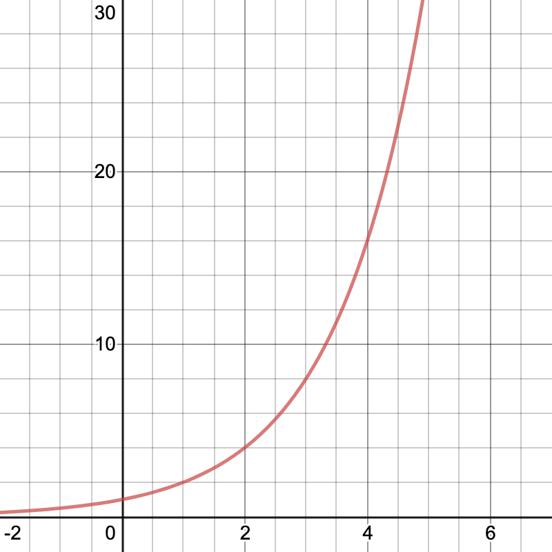
Notice that this graph is not a straight line; rather, it is a curve that has an increasing rate of change. That is, as the input (horizontal) values increase, the output (vertical) values increase at a faster and faster rate. This means the function f(x) cannot be linear, because its graph is not a straight line.

Now, we move onto the table b, which describes a function \(g(x)\). We notice that the inputs of \(g(x)\) change by \(1\), so the outputs should either increase or decrease at a constant rate. Indeed, as we move from \(g(1) = 4\) to \(g(2) = 1\), we decrease by \(3\). Then from \(g(2) = 1\) to \(g(3) = -2\), we decrease by 3 again. Likewise, from \(g(3) = -2\) to \(g(4) = -5\) is a decrease by 3.

Therefore, table b could represent a linear function. If we plot the points and connect them, we get the following graph:

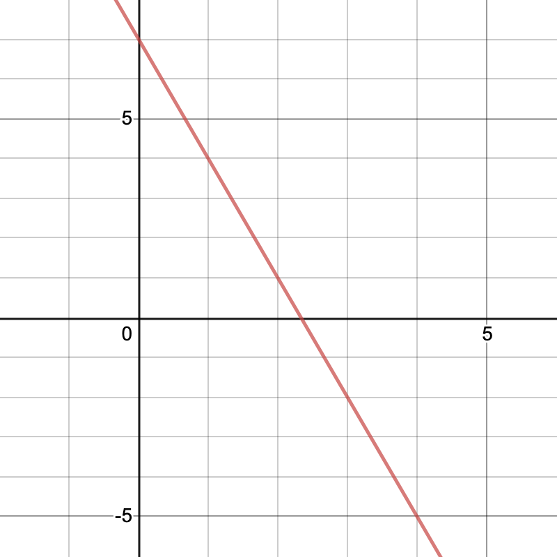
This graph is a straight line, which is further geometric confirmation that \(g(x)\) could be a linear function.

You may wonder how to take the data given in the previous example and make a linear function from it. There is a process to do this, which involves a slightly more careful look at the concept of slope.

Definition: Slope

The slope of a linear function is the rate of change of the linear function. That is, the slope is the constant amount of increase or decrease for each change of 1 to the input of the function. It is calculated as \[ m = \text{ slope } = \frac{\text{rise}}{\text{run}} = \frac{y_2 - y_1}{x_2 - x_1}\]

where \((x_1, y_1), (x_2, y_2)\) are any two points on the line.

Here is a brief explanation of the formula: we are comparing two points on the line, \((x_1, x_2)\) and \((y_1, y_2)\), and calculating the ratio of "change in \(y\)" to "change in \(x\)." To do that, we calculate \(y_2 - y_1\), which is the vertical distance between the two points, also known as the "rise." Likewise, the quantity \(x_2 - x_1\) is horizontal distance between the two points, also known as the "run". The slope is the ratio of these two quantities, read as "rise over run." It describes the change in the output \(y\) as it relates to the change in the input \(x\). An example will help illustrate this.

Example \(\PageIndex{4}\)

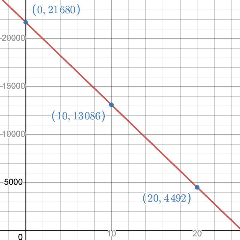
According to Honda's website, a new basic model 2013 Honda accord cost \(\$21,680\) when it was first sold. In 2023, such a car should sell for about \(\$13,086\) according to Kelly Blue Book. Assuming that the price of a 2013 Honda Accord changes linearly over time:

• Find the slope of the linear function describing the price of a Honda Accord, and interpret it in context.
• Find a formula for the linear function that describes the price of a Honda Accord \(t\) years after \(2013\) and interpret the vertical intercept in context.
• Use your function to predict the price of a Honda Accord sedan in \(2033\), and label the corresponding point on the graph.
• Find the year in which the price of a 2013 Honda Accord is projected to be \(\$7929.60\). 

Solution

First, please take note that this is an oversimplified situation. Used car prices, while they do tend to decrease over time, are affected by market factors that make their value highly variable and subject to fluctuation. This exercise shows how to use linear functions to get a ballpark idea, but this should not be mistaken for an exact prediction!

Our first step is to take our two data points and convert them into ordered pairs. Here, a convenient input variable will be the time \(t\) in years since \(2013\), and the output variable will be the price \(P(t)\) in dollars. Our first point will be \((0, 21680)\), which corresponds to the fact that \(0\) years after the year 2013, a Honda Accord cost \(\$21,680\). Our second point will be \((10, 13086)\), which corresponds to the fact that \(10\) years after 2013, that same Honda Accord should \(\$13,086\). This process of converting the written information into mathematical points is always the first step of the mathematical problem-solving process.

Now we can use these points to stand in for \((x_1, y_1)\) and \((x_2, y_2)\) in the slope formula. We have: \[(x_1, y_1) = (0, 21680) \quad \text{ and } \quad (x_2, y_2) = (10, 13086)\]

Next, we'll use the slope formula to find the slope: \[\text{slope } = \frac{y_2 - y_1}{x_2 - x_1} = \frac{13086- 21680 }{10-0} = \frac{-8594}{10} = -859.4\]

Therefore, the slope of the linear function is \(-859.4\). Since the slope was calculated by dividing a number of dollars by a number of years, its units are dollars per year. That is, the slope is \(-$859.40\) per year. This means that a 2013 Honda Accord loses value at a rate of \(\$859.40\) per year. (Such a value loss is known as depreciation.)

To answer the second part, we need to work backwards a bit. We observe that the vertical intercept will correspond to the year \(t = 0\), which in this case is the year 2013. We have that the value of the car in 2013 is \(\$21,680\). Therefore, our vertical intercept is \(21680\).

Now that we have our slope and vertical intercept, we can write the equation of the linear function describing the cost of a 2013 Honda Accord \(t\) years after 2013: \[C(t) = -859.4t + 21680\]

To answer the last part, we will note that 2033 is \(20\) years after 2013, and therefore it corresponds to the value \(t = 20\). Thus, we simply need to evaluate the function \(C(t)\) at the value \(t = 20\). We have: \[C(20) = -859.4 \times 20 + 21680 = 4492\]

That is, in the year 2033, a 2013 Honda Accord is predicted to be worth about \(\$4,492\).

We can visualize the line and the values at all three points in time by graphing the line and labeling the points:

Our last question asks us to find the year in which the projected price of a 2013 Honda Accord is equal to \(\$7929.60\). This is slightly different from the previous question in that, instead of knowing the year and finding the price, we are going backwards — we know the price, and we are trying to find the year in which that price occurred. That means that instead of plugging in a value for \(t\), we are instead plugging in a value for \(C(t)\) and then solving for \(t\). This will require two steps of algebra, but one of them is already familiar to you from a previous chapter. 

We'll start by plugging in our cost, \(\$7929.60\), for \(C(t)\): \[7929.60 = -859.4t + 21680\] Our goal is to isolate \(t\). In order to do that, we need to use the fact that subtraction undoes addition. In other words, we will subtract \(21680\) from both sides: \[7929.60 - 21680 = -859.4t + 21680 - 21680\] On the right side, we see that \(21680 - 21680 = 0\), so we are left with \[7929.60 - 21680 = -859.4t\] We can then perform the subtraction on the left side, which gives us a negative number: \[-13750.4 = -859.4t\] Now we have a situation that may look familiar from the previous chapter: we can use division undoes multiplication! We get \[t = \frac{-13750.4}{-859.4} = 16\] This tells us that when \(t = 16\), the price is equal to \(\$7929.60\). Rephrasing the answer in context, we see that in 2029 (which is \(16\) years after 2013), the price of a 2013 Honda Accord is \(\$7929.60\). See if you can find the corresponding point on the graph above! 

This shows the importance of linear functions in making predictions about the future. Of course, not all relationships are linear. But often linear functions give close-enough estimates for many situations, and are relatively simple to calculate. We'll see more of how linear functions are used in making predictions in the next section.

Exercises

1. Go to Monmouth Power and Light's website. Find the flat fee (basic charge + service charge) for electricity, and the cost per kilowatt hour (kwh). (Be careful not to round here — the numbers are quite small but the decimals matter!)
   1. Write a linear function \(C(k)\) that describes the cost of your Monmouth electric bill in dollars, in terms of the number of kilowatt hours k that are used.
   2. According to the EPA, The average American household uses \(886\) kilowatt hours of energy each month. Find the cost of your electric bill in Monmouth if you use \(886\) kilowatt hours of energy in a given month using the function \(C(k)\).
   3. Graph the function C(k) either by hand or using an electronic graphing tool such as Desmos. Label the point corresponding to your answer from the previous question on the graph.
2. Of the following three tables, one does not represent a function, one represents a function that is not linear, and one represents a linear function. Identify which table satisfies which properties. Explain your answer using at least 3 complete sentences.

   1. Input	Output
      1	4
      2	16
      3	64
      4	256

   2. Input	Output
      1	7.5
      2	5
      3	2.5
      4	0

   3. Input	Output
      1	3
      2	5
      3	7
      1	9

3. A population of deer in a forest is 87 in 2015, and 175 in 2023. Assuming that the deer population changes linearly:
   1. Find the linear function P(t) that describes the population of deer in the forest t years after 2015.
   2. Using your function from the previous part, predict the deer population in 2030. (Round to the nearest deer if applicable.)
   3. Find the year in which the deer population is projected to be 417 deer. 
   4. Graph your function either by hand or using Desmos, and label the point corresponding to your answer from the previous two parts. 
   5. What are some limitations to this model? What is unrealistic about it?