1.2: Angles and The Dot Product

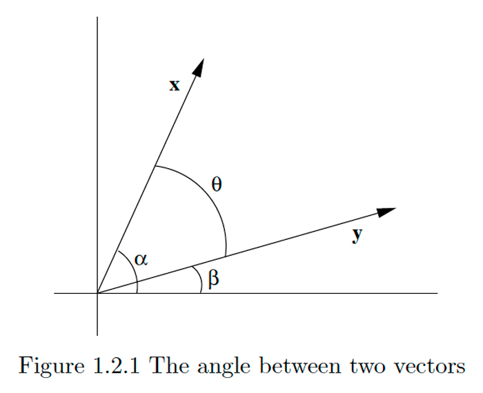
Suppose \(\mathbf{x}=\left(x_{1}, x_{2}\right)\) and \(\mathbf{y}=\left(y_{1}, y_{2}\right)\) are two vectors in \(\mathbf{R}^{2},\) neither of which is the zero vector \(\mathbf{0}\). Let \(\alpha\) and \(\beta\) be the angles between \(\mathbf{x}\) and \(\mathbf{y}\) and the positive horizontal axis, respectively, measured in the counterclockwise direction. Supposing \(\alpha \geq \beta,\) let \(\theta=\alpha-\beta\). Then \(\theta\) is the angle between \(\mathbf{x}\) and \(\mathbf{y}\) measured in the counterclockwise direction, as shown in Figure \(1.2 .1 .\) From the subtraction formula for cosine we have

\[\cos (\theta)=\cos (\alpha-\beta)=\cos (\alpha) \cos (\beta)+\sin (\alpha) \sin (\beta).\]

Now

\[\cos (\alpha)=\frac{x_{1}}{\|x\|},\]

\[\cos (\beta)=\frac{y_{1}}{\|\mathbf{y}\|},\]

\[\sin (\alpha)=\frac{x_{2}}{\|\mathbf{x}\|},\]

and

\[ \sin(\beta)=\frac{y_2}{\|\mathbf{y}\|}.\]

Thus, we have

\[\cos (\theta)=\frac{x_{1} y_{1}}{\|x\|\|y\|}+\frac{x_{2} y_{2}}{\|x\|\|y\|}=\frac{x_{1} y_{1}+x_{2} y_{2}}{\|x\|\|y\|}.\]

Example \(\PageIndex{1}\)

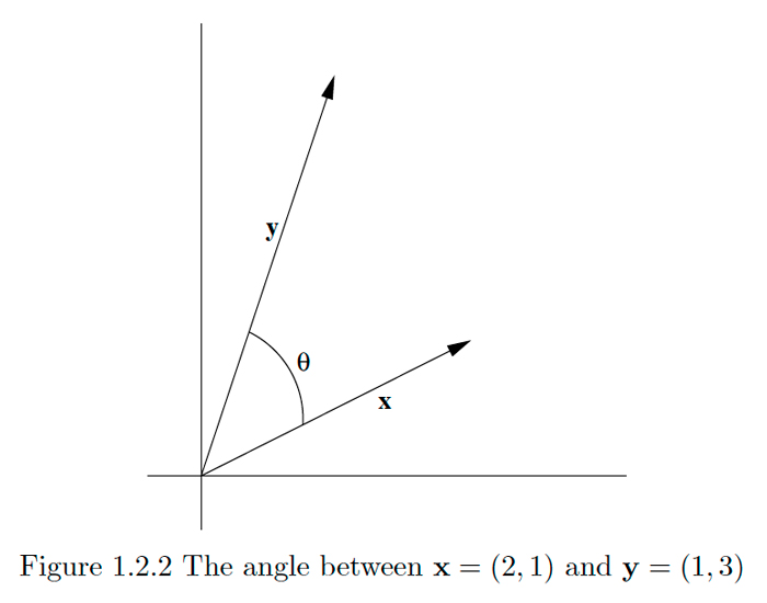
Let \(\theta\) be the smallest angle between \(\mathbf{x}=(2,1)\) and \(\mathbf{y}=(1,3),\) measured in the counterclockwise direction. Then, by \((1.2 .2),\) we must have

\[\cos (\theta)=\frac{(2)(1)+(1)(3)}{\|\mathbf{x}\|\|\mathbf{y}\|}=\frac{5}{\sqrt{5} \sqrt{10}}=\frac{1}{\sqrt{2}}.\]

Hence

\[\theta=\cos ^{-1}\left(\frac{1}{\sqrt{2}}\right)=\frac{\pi}{4}.\]

See Figure \(1.2 .2 .\)

With more work it is possible to show that if \(\mathbf{x}=\left(x_{1}, x_{2}, x_{3}\right)\) and \(\mathbf{y}=\left(y_{1}, y_{2}, y_{3}\right)\) are two vectors in \(\mathrm{R}^{3},\) neither of which is the zero vector \(\mathbb{0},\) and \(\theta\) is the smallest positive angle between \(x\) and \(y,\) then

\[\cos (\theta)=\frac{x_{1} y_{1}+x_{2} y_{2}+x_{3} y_{3}}{\|\mathbf{x}\|\|\mathbf{y}\|}\]

The term which appears in the numerators in both \((1.2 .2)\) and \((1.2 .3)\) arises frequently, so we will give it a name.

Definition

If \(\mathbf{x}=\left(x_{1}, x_{2}, \ldots, x_{n}\right)\) and \(\mathbf{y}=\left(y_{1}, y_{2}, \ldots, y_{n}\right)\) are vectors in \(\mathbb{R}^{n},\) then the dot product of \(\mathbf{x}\) and \(\mathbf{y},\) denoted \(\mathbf{x} \cdot \mathbf{y},\) is given by

\[\mathbf{x} \cdot \mathbf{y}=x_{1} y_{1}+x_{2} y_{2}+\cdots+x_{n} y_{n}.\]

Note that the dot product of two vectors is a scalar, not another vector. Because of this, the dot product is also called the scalar product. It is also an example of what is called an inner product and is often denoted by \(\langle\mathbf{x}, \mathbf{y}\rangle\).

Example \(\PageIndex{2}\)

If \(x=(1,2,-3,-2)\) and \(y=(-1,2,3,5),\) then

\[\mathbf{x} \cdot \mathbf{y}=(1)(-1)+(2)(2)+(-3)(3)+(-2)(5)=-1+4-9-10=-16.\]

The next proposition lists some useful properties of the dot product.

proposition \(\PageIndex{1}\)

For any vectors \(\mathbf{x}, \mathbf{y},\) and \(\mathbf{z}\) in \(\mathbb{R}^{n}\) and scalar \(\boldsymbol{\alpha}\),

\[\mathbf{x} \cdot \mathbf{y}=\mathbf{y} \cdot \mathbf{x},\]

\[\mathbf{x} \cdot(\mathbf{y}+\mathbf{z})=\mathbf{x} \cdot \mathbf{y}+\mathbf{x} \cdot \mathbf{z},\]

\[(\alpha \mathbf{x}) \cdot \mathbf{y}=\alpha(\mathbf{x} \cdot \mathbf{y}),\]

\[0 \cdot \mathbb{x}=0,\]

\[\mathbf{x} \cdot \mathbf{x} \geq 0,\]

\[\mathbf{x} \cdot \mathbf{x}=0 \text { only if } \mathbf{x}=\mathbf{0},\]

and

\[\mathbf{x} \cdot \mathbf{x}=\|\mathbf{x}\|^{2}.\]

These properties are all easily verifiable using the properties of real numbers and the definition of the dot product and will be left to Problem 9 for you to check.

At this point we can say that if \(x\) and \(y\) are two nonzero vectors in either \(\mathbb{R}^{2}\) or \(\mathbb{R}^{3}\) and \(\theta\) is the smallest positive angle between \(\mathbf{x}\) and \(\mathbf{y},\) then

\[\cos (\theta)=\frac{\mathbf{x} \cdot \mathbf{y}}{\|\mathbf{x}\|\|\mathbf{y}\|}.\]

We would like to be able to make the same statement about the angle between two vectors in any dimension, but we would first have to define what we mean by the angle between two vectors in \(\mathrm{R}^{n}\) for \(n>3 .\) The simplest way to do this is to turn things around and use \((1.2 .12)\) to define the angle. However, in order for this to work we must first know that
\[-1 \leq \frac{\mathbf{x} \cdot \mathbf{y}}{\|\mathbf{x}\|\|\mathbf{y}\|} \leq 1,\]
since this is the range of values for the cosine function. This fact follows from the following inequality.

Cauchy-Schwarz Inequality

For all \(x\) and \(y\) in \(\mathbb{R}^{n}\),
\[|\mathbf{x} \cdot \mathbf{y}| \leq\|\mathbf{x}\|\|\mathbf{y}\|.\]
To see why this is so, first note that both sides of \((1.2 .13)\) are 0 when \(y=0,\) and hence are equal in this case. Assuming \(\mathrm{x}\) and \(\mathrm{y}\) are fixed vectors in \(\mathbb{R}^{n},\) with \(\mathrm{y} \neq 0,\) let \(t\) be a real number and consider the function
\[f(t)=(\mathbf{x}+t \mathbf{y}) \cdot(\mathbf{x}+t \mathbf{y}).\]
By \((1.2 .9), f(t) \geq 0\) for all \(t,\) while from \((1.2 .6),(1.2 .7),\) and \((1.2 .11),\) we see that
\[f(t)=\mathbf{x} \cdot \mathbf{x}+\mathbf{x} \cdot t \mathbf{y}+t \mathbf{y} \cdot \mathbf{x}+t \mathbf{y} \cdot t \mathbf{y}=\|\mathbf{x}\|^{2}+2(\mathbf{x} \cdot \mathbf{y}) t+\|\mathbf{y}\|^{2} t^{2}.\]
Hence \(f\) is a quadratic polynomial with at most one root. Since the roots of \(f\) are, as given by the quadratic formula,
\[\frac{-2(\mathbf{x} \cdot \mathbf{y}) \pm \sqrt{4(\mathbf{x} \cdot \mathbf{y})^{2}-4\|\mathbf{x}\|^{2}\|\mathbf{y}\|^{2}}}{2\|\mathbf{y}\|^{2}},\]
it follows that we must have
\[4(\mathbf{x} \cdot \mathbf{y})^{2}-4\|\mathbf{x}\|^{2}\|\mathbf{y}\|^{2} \leq 0.\]
Thus
\[(\mathbf{x} \cdot \mathbf{y})^{2} \leq\|\mathbf{x}\|^{2}\|\mathbf{y}\|^{2},\]
and so
\[|\mathbf{x} \cdot \mathbf{y}| \leq\|\mathbf{x}\|\|\mathbf{y}\|.\]
Note that \(|\mathbf{x} \cdot \mathbf{y}|=\|\mathbf{x}\|\|\mathbf{y}\|\) if and only if there is some value of \(t\) for which \(f(t)=0,\) which, by \((1.2 .8)\) and \((1.2 .10),\) happens if and only if \(x+t y=0,\) that is, \(x=-t y,\) for some value of \(t .\) Moreover, if \(\mathbf{y}=\mathbf{0},\) then \(\mathbf{y}=0\mathbf{x}\), for any \(\mathbf{x}\) in \(\mathbb{R}^{n} .\) Hence, in either case, the Cauchy-Schwarz inequality becomes an equality if and only if either \(\mathbf{x}\) is a scalar multiple of \(\mathbf{y}\) or \(\mathbf{y}\) is a scalar multiple of \(\mathbf{x}\).
With the Cauchy-Schwarz inequality we have
\[-1 \leq \frac{\mathbf{x} \cdot \mathbf{y}}{\|\mathbf{x}\|\|\mathbf{y}\|} \leq 1\]
for any nonzero vectors \(\mathbf{x}\) and \(\mathbf{y}\) in \(\mathbb{R}^{n} .\) Thus we may now state the following definition.

Definition

If \(x\) and \(y\) are nonzero vectors in \(\mathbb{R}^{n},\) then we call
\[\theta=\cos ^{-1}\left(\frac{\mathbf{x} \cdot \mathbf{y}}{\|\mathbf{x}\|\|\mathbf{y}\|}\right)\]
the angle between \(\mathbf{x}\) and \(\mathbf{y} .\)

Example \(\PageIndex{3}\)

Suppose \(\mathbf{x}=(1,2,3)\) and \(\mathbf{y}=(1,-2,2) .\) Then \(\mathbf{x} \cdot \mathbf{y}=1-4+6=3,\|\mathbf{x}\|=\sqrt{14}\), and \(\|\mathbf{y}\|=3,\) so if \(\theta\) is the angle between \(\mathbf{x}\) and \(\mathbf{y},\) we have
\[\cos (\theta)=\frac{3}{3 \sqrt{14}}=\frac{1}{\sqrt{14}}.\]
Hence, rounding to four decimal places,
\[\theta=\cos ^{-1}\left(\frac{1}{\sqrt{14}}\right)=1.3002.\]

Example \(\PageIndex{4}\)

Suppose \(\mathbf{x}=(2,-1,3,1)\) and \(\mathbf{y}=(-2,3,1,-4) .\) Then \(\mathbf{x} \cdot \mathbf{y}=-8,\|\mathbf{x}\|=\sqrt{15}\), and \(\|\mathbf{y}\|=\sqrt{30},\) so if \(\theta\) is the angle between \(\mathbf{x}\) and \(\mathbf{y},\) we have, rounding to four decimal places,
\[\theta=\cos ^{-1}\left(\frac{-8}{\sqrt{15} \sqrt{30}}\right)=1.9575.\]

Example \(\PageIndex{5}\)

Let \(x\) be a vector in \(\mathbb{R}^{n}\) and let \(\alpha_{k}, k=1,2, \ldots, n,\) be the angle between \(x\) and the \(k\) th axis. Then \(\alpha_{k}\) is the angle between \(\mathbf{x}\) and the standard basis vector \(\mathbf{e}_{k} .\) Thus
\[\cos \left(\alpha_{k}\right)=\frac{\mathbf{x} \cdot \mathbf{e}_{k}}{\|\mathbf{x}\|\left\|\mathbf{e}_{k}\right\|}=\frac{x_{k}}{\|\mathbf{x}\|}.\]
That is, \(\cos \left(\alpha_{1}\right), \cos \left(\alpha_{2}\right), \ldots, \cos \left(\alpha_{n}\right)\) are the direction cosines of \(\mathbf{x}\) as defined in Section 1.1. For example, if \(\mathbf{x}=(3,1,2)\) in \(\mathbb{R}^{3},\) then \(\|\mathbf{x}\|=\sqrt{14}\) and the direction cosines of \(\mathbf{x}\) are
\[\begin{array}{l} {\cos \left(\alpha_{1}\right)=\frac{3}{\sqrt{14}}}, \\ {\cos \left(\alpha_{2}\right)=\frac{1}{\sqrt{14}}}, \end{array} \]
and
\[\cos \left(\alpha_{3}\right)=\frac{2}{\sqrt{14}},\]
giving us, to four decimal places,
\[\begin{array}{l} {\alpha_{1}=0.6405} \\ {\alpha_{2}=1.3002} \end{array}\]
and
\[\alpha_{3}=1.0069\]
Note that if \(x\) and \(y\) are nonzero vectors in \(\mathbb{R}^{n}\) with \(x \cdot y=0,\) then the angle between x and y is
\[\cos ^{-1}(0)=\frac{\pi}{2}.\]
This is the motivation behind our next definition.

Definition

Vectors \(\mathrm{x}\) and \(\mathrm{y}\) in \(\mathbb{R}^{n}\) are said to be orthogonal (or perpendicular), denoted \(\mathbf{x} \perp \mathbf{y},\) if \(\mathbf{x} \cdot \mathbf{y}=0\).

It is a convenient convention of mathematics not to restrict the definition of orthogonality to nonzero vectors. Hence it follows from the definition, and \((1.2 .8),\) that 0 is orthogonal to every vector in \(\mathbb{R}^{n} .\) Moreover, 0 is the only vector in \(\mathbb{R}^{n}\) which has this property, a fact you will be asked to verify in Problem 12.

Example \(\PageIndex{6}\)

The vectors \(\mathbf{x}=(-1,-2)\) and \(\mathbf{y}=(1,2)\) are both orthogonal to \(\mathbf{z}=(2,-1)\) in \(\mathbb{R}^{2} .\) Note that \(\mathbf{y}=-\mathbf{x}\) and, in fact, any scalar multiple of \(\mathbf{x}\) is orthogonal to z.

Example \(\PageIndex{7}\)

In \(\mathbb{R}^{4}, \mathbf{x}=(1,-1,1,-1)\) is orthogonal to \(\mathbf{y}=(1,1,1,1) .\) As in the previous example, any scalar multiple of \(\mathbf{x}\) is orthogonal to \(\mathbf{y}\).

Definition

We say vectors \(\mathbf{x}\) and \(\mathbf{y}\) are parallel if \(\mathbf{x}=\alpha \mathbf{y}\) for some scalar \(\alpha \neq 0\).

This definition says that vectors are parallel when one is a nonzero scalar multiple of the other. From our proof of the Cauchy-Schwarz inequality we know that it follows that if \(x\) and \(y\) are parallel, then \(|x \cdot y|=\|x\| \| y | .\) Thus if \(\theta\) is the angle between \(x\) and \(y\),
\[\cos (\theta)=\frac{\mathbf{x} \cdot \mathbf{y}}{\|\mathbf{x}\|\|\mathbf{y}\|}=\pm 1.\]
That is, \(\theta=0\) or \(\theta=\pi .\) Put another way, \(x\) and \(y\) either point in the same direction or they point in opposite directions.

Example \(\PageIndex{8}\)

The vectors \(x=(1,-3)\) and \(y=(-2,6)\) are parallel since \(x=-\frac{1}{2} y .\) Note that \(\mathbf{x} \cdot \mathbf{y}=-20\) and \(\|\mathbf{x}\|\|\mathbf{y}\|=\sqrt{10} \sqrt{40}=20,\) so \(\mathbf{x} \cdot \mathbf{y}=-\|\mathbf{x}\|\|\mathbf{y}\| .\) It follows that the angle between \(x\) and \(y\) is \(\pi\).

Two basic results about triangles in \(\mathbb{R}^{2}\) and \(\mathbb{R}^{3}\) are the triangle inequality (the sum of the lengths of two sides of a triangle is greater than or equal to the length of the third side \()\) and the Pythagorean theorem (the sum of the squares of the lengths of the legs of a right triangle is equal to the square of the length of the other side). In terms of vectors in \(\mathbb{R}^{n},\) if we picture a vector \(\mathbf{x}\) with its tail at the origin and a vector \(\mathbf{y}\) with its tail at the tip of \(\mathbf{x}\) as two sides of a triangle, then the remaining side is given by the vector \(\mathbf{x}+\mathbf{y}\). Thus the triangle inequality may be stated as follows.

Triangle inequality

If \(x\) and \(y\) are vectors in \(\mathbb{R}^{n},\) then
\[\|\mathbf{x}+\mathbf{y}\| \leq\|\mathbf{x}\|+\|\mathbf{y}\|.\]
The first step in verifying \((1.2 .21)\) is to note that, using \((1.2 .11)\) and \((1.2 .6)\),
\[ \begin{aligned} \|\mathbf{x}+\mathbf{y}\|^{2} &=(\mathbf{x}+\mathbf{y}) \cdot(\mathbf{x}+\mathbf{y}) \\ &=\mathbf{x} \cdot \mathbf{x}+2(\mathbf{x} \cdot \mathbf{y})+\mathbf{y} \cdot \mathbf{y} \\ &=\|\mathbf{x}\|^{2}+2(\mathbf{x} \cdot \mathbf{y})+\|\mathbf{y}\|^{2} \end{aligned}\]
Since \(\mathbf{x} \cdot \mathbf{y} \leq\|\mathbf{x}\|\|\mathbf{y}\|\) by the Cauchy-Schwarz inequality, it follows that
\[\|\mathbf{x}+\mathbf{y}\|^{2} \leq \| \mathbf{x}\left\|^{2}+2\right\| \mathbf{x}\|\| \mathbf{y}\|+\| \mathbf{y}\left\|^{2}=(\|\mathbf{x}\|+\|\mathbf{y}\|)^{2}\right.\]
from which we obtain the triangle inequality by taking square roots.
Note that in \((1.2 .22)\) we have
\[\|\mathbf{x}+\mathbf{y}\|^{2}=\|\mathbf{x}\|^{2}+\|\mathbf{y}\|^{2}\]
if and only if \(x \cdot y=0,\) that is, if and only if \(x \perp y .\) Hence we have the following famous result.

Pythagorean theorem

Vectors \(\mathbf{x}\) and \(\mathbf{y}\) in \(\mathbb{R}^{n}\) are orthogonal if and only if
\[\|\mathbf{x}+\mathbf{y}\|^{2}=\|\mathbf{x}\|^{2}+\|\mathbf{y}\|^{2}.\]

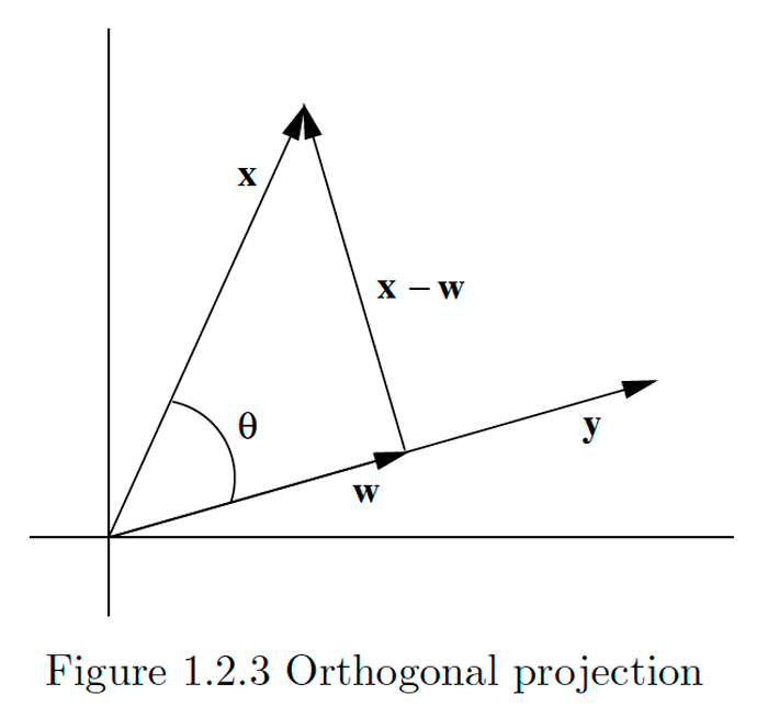
Perhaps the most important application of the dot product is in finding the orthogonal projection of one vector onto another. This is illustrated in Figure \(1.2 .3,\) where w represents the projection of \(x\) onto \(y .\) The result of the projection is to break \(x\) into the sum of two components, \mathbf{w}, which is parallel to \(\mathbf{y},\) and \(\mathbf{x}-\mathbf{w},\) which is orthogonal to \(\mathbf{y},\) a procedure which is frequently very useful. To compute \mathbf{w}, note that if \(\theta\) is the angle between \(\mathbf{x}\) and \(\mathbf{y},\) then
\[\|\mathbf{w}\|=\|\mathbf{x}\|\left|\cos (\theta)\left|=\|\mathbf{x}\| \frac{|\mathbf{x} \cdot \mathbf{y}\|}{\|\mathbf{x}\|\|\mathbf{y}\|}=\right| \mathbf{x} \cdot \frac{\mathbf{y}}{\|\mathbf{y}\|}\right|=| \mathbf{x} \cdot \mathbf{u} |,\]
where
\[\mathbf{u}=\frac{\mathbf{y}}{\|\mathbf{y}\|}\]
is the direction of \(\mathbf{y} .\) Hence \(\mathbf{w}=|\mathbf{x} \cdot \mathbf{u}| \mathbf{u}\) when \(0 \leq \theta \leq \frac{\pi}{2},\) which is when \(\mathbf{x} \cdot \mathbf{u}>0,\) and
\(\mathbf{w}=-|\mathbf{x} \cdot \mathbf{u}| \mathbf{u}\) when \(\frac{\pi}{2}<\theta \leq \pi,\) which is when \(\mathbf{x} \cdot \mathbf{u}<0 .\) Thus, in either case, \(\mathbf{w}=(\mathbf{x} \cdot \mathbf{u}) \mathbf{u}\).

Definition

Given vectors \(\mathbf{x}\) and \(\mathbf{y}, \mathbf{y} \neq \mathbf{0},\) in \(\mathbb{R}^{n},\) the vector
\[\mathbf{w}=(\mathbf{x} \cdot \mathbf{u}) \mathbf{u},\]
where \(\mathbf{u}\) is the direction of \(\mathbf{y},\) is called the orthogonal projection, or simply projection, of \(\mathbf{x}\) onto y. We also call w the component of \(x\) in the direction of \(y\) and \(x \cdot u\) the coordinate of \(x\) in the direction of \(y .\)

In the special case where \(\mathrm{y}=\mathbf{e}_{k},\) the \(k\) th standard basic vector, \(k=1,2, \ldots, n,\) we see that the coordinate of \(\mathbf{x}=\left(x_{1}, x_{2}, \ldots, x_{n}\right)\) in the direction of \(y\) is just \(x \cdot e_{k}=x_{k},\) the \(k\) th coordinate of \(\mathbf{x}\).

Example \(\PageIndex{9}\)

Suppose \(\mathbf{x}=(1,2,3)\) and \(\mathbf{y}=(1,4,0) .\) Then the direction of \(\mathbf{y}\) is
\[\mathbf{u}=\frac{1}{\sqrt{17}}(1,4,0),\]
so the coordinate of \(x\) in the direction of \(y\) is
\[\mathbf{x} \cdot \mathbf{u}=\frac{1}{\sqrt{17}}(1+8+0)=\frac{9}{\sqrt{17}}.\]
Thus the projection of \(x\) onto \(y\) is
\[\mathbf{w}=\frac{9}{\sqrt{17}} \mathbf{u}=\frac{9}{17}(1,4,0)=\left(\frac{9}{17}, \frac{36}{17}, 0\right).\]