5.2: Taylor Series

For Real Functions

Let \(a\in \mathbb R\) and \(f(x)\) be and infinitely differentiable function on an interval \(I\) containing \(a\). Then the one-dimensional Taylor series of \(f\) around \(a\) is given by

\(f(x)=f(a)+f’(a)(x-a)+\frac{f’’(a)}{2!}(x-a)^2+\frac{f^{(3)}(a)}{3!}(x-a)^3+\cdots\)

which can be written in the most compact form:

\(f(x)=\sum_{n=0}^{\infty} \frac{f^{(n)}(a)}{n!}(x-a)^n.\)

Recall that, in real analysis, Taylor’s theorem gives an approximation of a \(k\)-times differentiable function around a given point by a \(k\)-th order Taylor polynomial.

For example, the best linear approximation for \(f(x)\) is

\(f(x)\approx f(a)+f′(a)(x−a).\)

This linear approximation fits \(f(x)\) with a line through \(x=a\) that matches the slope of \(f\) at \(a\).

For a better approximation we can add other terms in the expansion. For instance, the best quadratic approximation is

\(f(x)\approx f(a)+f’(a)(x−a)+\frac12 f’’(a)(x−a)^2.\)

The following applet shows the partial sums of the Taylor series for a given function. Drag the slider to show more terms of the series. Drag the point a or change the function.

 

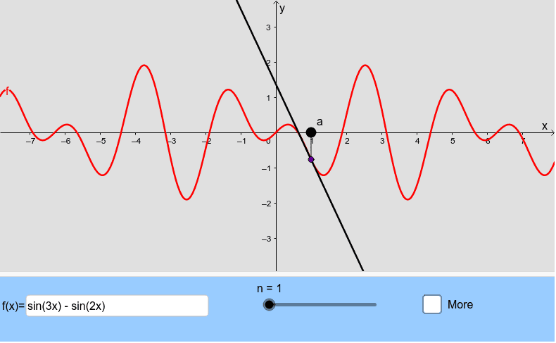
INTERACTIVE GRAPH

 

---

For Complex Functions

Suppose that a function \(f\) is analytic throughout a disk \(|z -z_0|< R\), centred at \(z_0\) and with radius \(R_0\). Then \(f(z)\) has the power series representation

\(\begin{eqnarray}\label{seriefunction}
                f(z)=\sum_{n=0}^{\infty} a_n(z-z_0)^n,\quad |z-z_0|<R,
                \end{eqnarray}\)

where

\(\begin{eqnarray}
                a_n=\frac{f^{(n)}(z_0)}{n!},\quad n=0,1,2,\ldots
                \end{eqnarray}
\)

That is, series (1) converges to \(f(z)\) when \(z\) lies in the stated open disk.

Every complex power series (1) has a radius of convergence. Analogous to the concept of an interval of convergence for real power series, a complex power series (1) has a circle of convergence, which is the circle centered at \(z_0\) of largest radius \(R>0\) for which (1) converges at every point within the circle \(|z−z_0|=R\). A power series converges absolutely at all points \(z\) within its circle of convergence, that is, for all \(z\) satisfying \(|z−z_0|<R\), and diverges at all points \(z\) exterior to the circle, that is, for all \(z\) satisfying \(|z−z_0|>R\). The radius of convergence can be:

1. \(R=0\) (in which case (1) converges only at its center \(z=z_0\)),
2. \(R\) a finite positive number (in which case (1) converges at all interior points of the circle \(|z−z_0|<R\), or
3. \(R=∞\) (in which case (1) converges for all \(z\)).

The radius of convergence can be calculated using the ratio test of convergece. For example, if:

1. \(\displaystyle \lim_{n\rightarrow \infty} \left| \frac{a_{n+1}}{a_n}\right| = L\neq 0\), the radius of convergence is \(R=\dfrac{1}{L}\);
2. \(\displaystyle \lim_{n\rightarrow \infty}  \left| \frac{a_{n+1}}{a_n}\right|= 0\), the radius of convergence is \(R=∞\);
3. \(\displaystyle \lim_{n\rightarrow \infty}  \left| \frac{a_{n+1}}{a_n}\right|= \infty\), the radius of convergence is \(R=0\).

---

Dynamic Exploration

Use the following applet to explore Taylor series representations and its radius of convergence which depends on the value of \(z_0\).

On the left side of the applet below, a phase portrait of a complex function is displayed. On the right side, you can see the approximation of the function through it’s Taylor polynomials at the blue base point \(z_0\). The complex function, the base point \(z_0\), the order of the polynomial (vertical slider) and the zoom (horizontal slider) can be modified.

 

INTERACTIVE GRAPH

 

 

---

Maclaurin series

A Taylor series with centre \(z_0=0\)

\(f(z) = \sum_{n=0}^{\infty} \frac{f^{(n)}(0)}{n!}z^n\)

is referred to as Maclaurin series.

Some important Maclaurin series are:

\(\begin{eqnarray*}
            \displaystyle \frac{1}{1-z}&=& \sum_{n=0}^{\infty} z^n, \quad |z|\lt 1; \\
            \displaystyle e^z &=& \sum_{n=0}^{\infty} \frac{z^n}{n!} \quad |z|\lt \infty;\\
            \displaystyle \sin z &=& \sum_{n=0}^{\infty} (-1)^n\frac{z^{2n+1}}{n!} \quad |z|\lt \infty;\\
            \displaystyle \cos z &=& \sum_{n=0}^{\infty} (-1)^n \frac{z^{2n}}{n!} \quad |z|\lt \infty;\\
            \displaystyle \sinh z &=& \sum_{n=0}^{\infty} \frac{z^{2n+1}}{n!} \quad |z|\lt \infty;\\
            \displaystyle \cosh z &=& \sum_{n=0}^{\infty} \frac{z^{2n}}{n!} \quad |z|\lt \infty;
            \end{eqnarray*}\)

Exercise \(\PageIndex{1}\)

Exercise: Find the Maclaurin series expansion of the function

\(f(z)=\frac{z}{z^4+9}\)

and calculate the radius of convergence.

---

Note

The applet was originally written by Aaron Montag using CindyJS. The source can be found at GitHub.