
part0002
- Page ID
- 24588
\( \newcommand{\vecs}[1]{\overset { \scriptstyle \rightharpoonup} {\mathbf{#1}} } \)
\( \newcommand{\vecd}[1]{\overset{-\!-\!\rightharpoonup}{\vphantom{a}\smash {#1}}} \)
\( \newcommand{\id}{\mathrm{id}}\) \( \newcommand{\Span}{\mathrm{span}}\)
( \newcommand{\kernel}{\mathrm{null}\,}\) \( \newcommand{\range}{\mathrm{range}\,}\)
\( \newcommand{\RealPart}{\mathrm{Re}}\) \( \newcommand{\ImaginaryPart}{\mathrm{Im}}\)
\( \newcommand{\Argument}{\mathrm{Arg}}\) \( \newcommand{\norm}[1]{\| #1 \|}\)
\( \newcommand{\inner}[2]{\langle #1, #2 \rangle}\)
\( \newcommand{\Span}{\mathrm{span}}\)
\( \newcommand{\id}{\mathrm{id}}\)
\( \newcommand{\Span}{\mathrm{span}}\)
\( \newcommand{\kernel}{\mathrm{null}\,}\)
\( \newcommand{\range}{\mathrm{range}\,}\)
\( \newcommand{\RealPart}{\mathrm{Re}}\)
\( \newcommand{\ImaginaryPart}{\mathrm{Im}}\)
\( \newcommand{\Argument}{\mathrm{Arg}}\)
\( \newcommand{\norm}[1]{\| #1 \|}\)
\( \newcommand{\inner}[2]{\langle #1, #2 \rangle}\)
\( \newcommand{\Span}{\mathrm{span}}\) \( \newcommand{\AA}{\unicode[.8,0]{x212B}}\)
\( \newcommand{\vectorA}[1]{\vec{#1}} % arrow\)
\( \newcommand{\vectorAt}[1]{\vec{\text{#1}}} % arrow\)
\( \newcommand{\vectorB}[1]{\overset { \scriptstyle \rightharpoonup} {\mathbf{#1}} } \)
\( \newcommand{\vectorC}[1]{\textbf{#1}} \)
\( \newcommand{\vectorD}[1]{\overrightarrow{#1}} \)
\( \newcommand{\vectorDt}[1]{\overrightarrow{\text{#1}}} \)
\( \newcommand{\vectE}[1]{\overset{-\!-\!\rightharpoonup}{\vphantom{a}\smash{\mathbf {#1}}}} \)
\( \newcommand{\vecs}[1]{\overset { \scriptstyle \rightharpoonup} {\mathbf{#1}} } \)
\( \newcommand{\vecd}[1]{\overset{-\!-\!\rightharpoonup}{\vphantom{a}\smash {#1}}} \)
\(\newcommand{\avec}{\mathbf a}\) \(\newcommand{\bvec}{\mathbf b}\) \(\newcommand{\cvec}{\mathbf c}\) \(\newcommand{\dvec}{\mathbf d}\) \(\newcommand{\dtil}{\widetilde{\mathbf d}}\) \(\newcommand{\evec}{\mathbf e}\) \(\newcommand{\fvec}{\mathbf f}\) \(\newcommand{\nvec}{\mathbf n}\) \(\newcommand{\pvec}{\mathbf p}\) \(\newcommand{\qvec}{\mathbf q}\) \(\newcommand{\svec}{\mathbf s}\) \(\newcommand{\tvec}{\mathbf t}\) \(\newcommand{\uvec}{\mathbf u}\) \(\newcommand{\vvec}{\mathbf v}\) \(\newcommand{\wvec}{\mathbf w}\) \(\newcommand{\xvec}{\mathbf x}\) \(\newcommand{\yvec}{\mathbf y}\) \(\newcommand{\zvec}{\mathbf z}\) \(\newcommand{\rvec}{\mathbf r}\) \(\newcommand{\mvec}{\mathbf m}\) \(\newcommand{\zerovec}{\mathbf 0}\) \(\newcommand{\onevec}{\mathbf 1}\) \(\newcommand{\real}{\mathbb R}\) \(\newcommand{\twovec}[2]{\left[\begin{array}{r}#1 \\ #2 \end{array}\right]}\) \(\newcommand{\ctwovec}[2]{\left[\begin{array}{c}#1 \\ #2 \end{array}\right]}\) \(\newcommand{\threevec}[3]{\left[\begin{array}{r}#1 \\ #2 \\ #3 \end{array}\right]}\) \(\newcommand{\cthreevec}[3]{\left[\begin{array}{c}#1 \\ #2 \\ #3 \end{array}\right]}\) \(\newcommand{\fourvec}[4]{\left[\begin{array}{r}#1 \\ #2 \\ #3 \\ #4 \end{array}\right]}\) \(\newcommand{\cfourvec}[4]{\left[\begin{array}{c}#1 \\ #2 \\ #3 \\ #4 \end{array}\right]}\) \(\newcommand{\fivevec}[5]{\left[\begin{array}{r}#1 \\ #2 \\ #3 \\ #4 \\ #5 \\ \end{array}\right]}\) \(\newcommand{\cfivevec}[5]{\left[\begin{array}{c}#1 \\ #2 \\ #3 \\ #4 \\ #5 \\ \end{array}\right]}\) \(\newcommand{\mattwo}[4]{\left[\begin{array}{rr}#1 \amp #2 \\ #3 \amp #4 \\ \end{array}\right]}\) \(\newcommand{\laspan}[1]{\text{Span}\{#1\}}\) \(\newcommand{\bcal}{\cal B}\) \(\newcommand{\ccal}{\cal C}\) \(\newcommand{\scal}{\cal S}\) \(\newcommand{\wcal}{\cal W}\) \(\newcommand{\ecal}{\cal E}\) \(\newcommand{\coords}[2]{\left\{#1\right\}_{#2}}\) \(\newcommand{\gray}[1]{\color{gray}{#1}}\) \(\newcommand{\lgray}[1]{\color{lightgray}{#1}}\) \(\newcommand{\rank}{\operatorname{rank}}\) \(\newcommand{\row}{\text{Row}}\) \(\newcommand{\col}{\text{Col}}\) \(\renewcommand{\row}{\text{Row}}\) \(\newcommand{\nul}{\text{Nul}}\) \(\newcommand{\var}{\text{Var}}\) \(\newcommand{\corr}{\text{corr}}\) \(\newcommand{\len}[1]{\left|#1\right|}\) \(\newcommand{\bbar}{\overline{\bvec}}\) \(\newcommand{\bhat}{\widehat{\bvec}}\) \(\newcommand{\bperp}{\bvec^\perp}\) \(\newcommand{\xhat}{\widehat{\xvec}}\) \(\newcommand{\vhat}{\widehat{\vvec}}\) \(\newcommand{\uhat}{\widehat{\uvec}}\) \(\newcommand{\what}{\widehat{\wvec}}\) \(\newcommand{\Sighat}{\widehat{\Sigma}}\) \(\newcommand{\lt}{<}\) \(\newcommand{\gt}{>}\) \(\newcommand{\amp}{&}\) \(\definecolor{fillinmathshade}{gray}{0.9}\)F = k 2 d 2 (1 – kd) Find the value of d that will maximize the amount of food gathered.
CHAPTER 3. THE DERIVATIVE
162
3.6 The second derivative and higher order derivatives.
You may read or hear statements such as “the rate of population growth is decreasing”, or “the rate of inflation is increasing”, or the velocity of the particle is increasing.” In each case the underlying quantity is a rate and its rate of change is important.
Definition 3.6.1 The second derivative. The second derivative of a function, P, is the derivative of the derivative of P, or the derivative of P’.
The second derivative of P may be denoted by
P”, P”(t), ~ P, P(t), P^\ pM(t), or DlP{t)
Geometry of the first and second derivatives. That a function, P is increasing on an interval [a, b] means that
if s and t are in [a, b] and s < t then P(s) < P{t)
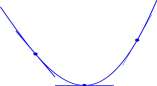
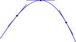
It should be fairly intuitive that if the first derivative of a function, P, is positive throughout [a, b], then P is increasing on [a, b]. Both graphs in Figure 3.24 have positive first derivatives and are increasing. The graphs also illustrate the geometry of the second derivative. In Figure 3.24A P’ is increasing (P'(s) < P'(t)). P has a positive second derivative (P” > 0) and the graph of P is concave upward. In Figure 3.24B, P’ is decreasing (P'(s) > P'(t)). P has a negative second derivative (P” < 0) and the graph of P is concave downward. We will expand on this interpretation in Chapters 8 and 12.
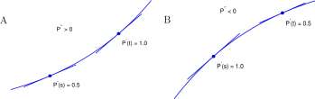
s < t s < t
Figure 3.24: A. Graph of a function with a positive second derivative; it is concave up. B. Graph of a function with a negative second derivative; it is concave down.
The higher order derivatives are a natural extension of the transition from the derivative to the second derivative. The third derivative is the derivative of the second derivative; the fourth derivative is the derivative of the third derivative; and the process continues. In this language, the
CHAPTER 3. THE DERIVATIVE
163
derivative of P is called the first derivative of P (and sometimes P itself is called the zero-order derivative of P).
Definition 3.6.2 Inductive definition of higher order derivatives. The
derivative of a function, P, is the order 1 derivative of P. For n an integer greater than 1, the order n derivative of P is the derivative of the order n — 1 derivative of P.
The third order derivative of P may be denoted by
P>”, P”‘(t), ^, p( 3 >, P( 3 )(t), or P 3 P(t)
For n > 3 the nth order derivative of P may be denoted by
d n P
P (n \ P (n) (t), —, or D?P(t)
If P(t) — fjt + (3 is a linear function, then p'(t) = u, is a constant function, and P”(t) = [u] = 0 is the zero function. A similar pattern occurs with quadratic polynomials. Suppose P(t) = at 2 + bt + c is a quadratic polynomial. Then
P'{t) = [at 2 + bt + c]’
= 2 at + b P'(t) is a linear function.
P”(t) = [2at + b]’
(3.35)
= 2 a P”(t) i s a constant function.
P'”(t) = [2 a]’
= 0 P”‘(t) is the zero function.
Explore 3.6.1 Suppose P(t) = a + bt + ct 2 + dt 3 is a cubic polynomial. Show that P’ is a quadratic polynomial, P” is a linear function, P'” is a constant function, and P^ is the zero function.
If S(t) is the position of a particle along an axis at time t, then s'(t) is the velocity of the particle and the rate of change of velocity, s”(t), is called the acceleration of the particle. Sometimes when s”(t) is negative the word deceleration is used to describe the motion of the particle. The word acceleration is used to describe second derivatives in other contexts. An accelerating economy is one in which the rate of increase of the gross national product is increasing.
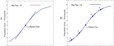
Example 3.6.1 Shown in Figure 3.25A is the graph of the logistic function, L(t), first shown in Figure 3.15. Some tangents are drawn on the graph of L. The slope at b is greater than the slope at a; the slope, L'(t), is increasing on the interval to the left of the point marked, i= Inflect ion Point.
CHAPTER 3. THE DERIVATIVE
164
012345678 01234567
Time – Years Time – Years
Figure 3.25: A. The graph of a logistic equation and an inflection point /. B. The same graph with tangent segments. The slope of the segment at a is less than the slope at b. The slope at c is greater than the slope at d.
Explore 3.6.2 Do this.
a. The slopes of L at b and d are approximately 1.5 and 0.75. Estimate the slopes at a and c. Confirm that the slope at a is less than the slope at b and that the slope at c is greater than the slope at d.
b. Let ti be the time of the inflection point /. Argue that L”(t) > 0 on [0,ij].
c. Argue that L”(t) < 0 for t > U.
d. Argue that L”(tj) = 0.
e. On what interval is the graph of L concave downward?^
The tangent at the inflection point is shown in Figure 3.25B, and it is interesting that the tangent crosses the curve at I. The slope of that tangent = 1.733, and is the largest of the slopes of all of the tangents. The maximum population growth rate occurs at ti and is approximately 1733 individuals per year.
Explore 3.6.3 Danger: Obnubilation Zone. You have to think about this. Suppose the population represented by the logistic curve in Figure 3.25 is a natural population such as deer, fish, geese or shrimp, and suppose you are responsible for setting the size of harvest each year. What is your strategy?
Argue with a friend about this. You should observe that the population size at the inflection point, I, is 5 which is one-half the maximum supportable population of 10. You should discuss the fact that variable weather, disease and other factors may disrupt the ideal of logistic growth. You should discuss how much harvest you could have if you maintained the population at points a, b, c or d in Figure 3.25A. ■
CHAPTER 3. THE DERIVATIVE
165
3.6.1 Falling objects.
We describe the position, s(t), of an object falling in the earth’s gravity field near the Earth’s surface t seconds after release. We assume that the velocity of the object at time of release is vq and the height of the object above the earth (or some reference point) at time of release is sq. Gravity near the Earth’s surface is constant, equal to g = -980 cm/sec 2 . We write the
Mathematical Model 3.6.1 Free falling object. The acceleration of a free falling object near the Earth’s surface is the acceleration of gravity, g.
Because s”(t) is the acceleration of the falling object, we write
s”(t) = g.
Now, s” is a constant and is the derivative of s’. The derivative of a linear function, P(t) = at + b, is a constant (P'(t) = a). We invoke some advertising logic 9 and guess that s'{t) is a linear function (proved in Chapter 10).
s'(t) = gt + b Bolt out of Chapter 10.
Because s'(0) = fo is assumed known, and s'(0) = g 0 + b = b, we write
s'(t) = gt + s 0
Using equally compelling logic, because the derivative of a quadratic function, Pit) = at 2 + bt + c, is a linear function (P'(t) = 2at + b), and because s’ is a linear function and s(0) = s 0 , we write
s(t) = ^t 2 + v 0 t + s 0 (3.36)
Example 3.6.2 Students measured height vs time of a falling bean bag using a Texas Instruments Calculator Based Laboratory Motion Detector, and the data are shown in Figure 3.26A. Average velocities were computed between data points and plotted against the midpoints of the data intervals in Figure 3.26B. Mid-time is (Timej + i + Timej)/2 and Ave. Vel. is (Heightj+i -Height;)/(Time m – Time*).
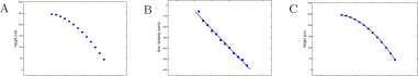
Time (b) Mid Time (s) Time (s)
Figure 3.26: Graph of height vs time and velocity vs time of a falling bean bag.
An equation of the line fit by least squares to the graph of Average Velocity vs Midpoint of time interval is
^ave = -849t mid + 126 cm/s.
9 Advertising Logic: A tall, muscular, rugged man drives a Dodge Ram. If you buy a Dodge Ram, you will be a tall muscular, rugged man.
CHAPTER 3. THE DERIVATIVE
166
If we assume a continuous model based on this data, we have
—849
s'(t) = -8491 + 126, s(t) = —— t 2 + 126 t + s 0 cm
From Figure 3.26, the height of the first point is about 240. We write
—849
s(t) = —— t 2 + 1261 +240 cm
The graph of s along with the original data is shown in Figure 3.26C. The match is good. Instead of g -980 cm/s 2 that applies to objects falling in a vacuum we have acceleration of the bean bag in air to be —849cm/sec 2 . h
Exercises for Section 3.6, The second derivative and higher order derivatives.
Exercise 3.6.1 Compute P’, P” and P'” for the following functions.
a. P{t) = 17 b. P{t) = t c. P(t) = t 2
d. P(t) = t 3 e. P(t) = t 1 / 2 f. P(t) = t1
g. P(t) = t 8 h. P(t) = t 125 i. P(t) = t 5 ^ 2
Exercise 3.6.2 Find the acceleration of a particle at time t whose position, Pit), on an axis is described by
a. P(t) = 15 b. P(t) = 5t + 7
c. P(t) = -4.9t 2 + 22t + 5 d. P(t) = t-^ + j^j
Exercise 3.6.3 Compute P’, P” and P'” and ?W for P{t) = a + bt + ct 2 + dt 3 .
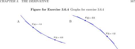
Exercise 3.6.4 For each figure in Exercise Figure 3.6.4, state whether:
a. P is increasing or decreasing?
b. P’ is positive or negative?
c. P’ is increasing or decreasing?
d. P”{a) positive or negative?
e. The graph of P is concave up or concave down
S < t S < t
Exercise 3.6.5 The function, P, graphed in Figure Ex. 3.6.5 has a local minimum at the point
(a,P(a)).
a. What is P'{a)1
b. For t < a, P'(t) is (positive or negative)?
c. For a < t, P'(t) is (positive or negative)?
d. P'(t) is (increasing or decreasing)?
e. P”(a) is (positive or negative)?
Figure for Exercise 3.6.5 Graph of a function P with a minimum at (a,P(a)).
See Exercise 3.6.5.
(a, P(a»
Exercise 3.6.6 The function, P, graphed in Figure Ex. 3.6.6 has a local maximum at the point (a,P(a)).
a. What is P'(a)?
b. For t < a, P'(t) is (positive or negative)?
c. For a < t, P'(t) is (positive or negative)?
d. P'(t) is (increasing or decreasing)?
e. P”{a) is (positive or negative)?
CHAPTER 3. THE DERIVATIVE
168
Figure for Exercise 3.6.6 Graph of a function P with a maximum at (a,P(a)). See
Exercise 3.6.6.
(a, P(a))
Exercise 3.6.7 Show that A(t) of Equation 3.26,
A(t) = ^-t + 2j t>0,
satisfies Equation 3.25,
A{0) = 4 A'(t) = K^A(t) t > 0 You will need to compute A'(t) and to do so expand
A(t)= + to A(t) = B ^-t 2 + Kt + A
and show that
A , {t)=K(^t + 2^=K^Mt).
Exercise 3.6.8 Show that for s(t) = ft 2 + v 0 t + 7, s'(t) = gt + v 0 -Exercise 3.6.9 Evaluate 7 if
CHAPTER 3. THE DERIVATIVE Exercise 3.6.10 Show that
169
For parts g – k, use the Definition of Derivative 3.2.2 to compute P’. Exercise 3.6.11 Add the equations,
H 2 — Hi =
-849
if3 — Ho =
-849
(t 2 2 -tl) + 126(f 2 -*i) (t 2 3 -t 2 2 ) + 126(f 3 -t 2 )
H n -H n _ x = (t\-tl_ x ) + 126(t n -t n _i).
to obtain
—849 / \ H n -H 1 = — ( t 2 n – t\ ) + 126 ( t n – h ).
Exercise 3.6.12 In a chemical reaction of the form
2A + B —► A 2 B,
where the reaction does not involve intermediate compounds, the reaction rate is proportional to [A] 2 [B] where [A] and [B] denote, respectively, the concentrations of the components A and B. Let a and b denote [A] and [B], respectively, and assume that [B] is much greater than [A] so that (b(t) 3> a(t). The rate at which a changes may be written
a’it) = -k i a(t) f bit) = -K ( a(t) f
CHAPTER 3. THE DERIVATIVE
170
We have assumed that b(t) is (almost) constant because [A] is the limiting concentration of the reaction. Let
a(t)
a 0
1 — a 0 K t
Show that a(0) = a Q .
Use the Definition of Derivative 3.22,
a'(t) = lim
a(b) — a(t)
t b-t
to compute a'(t). Then compute (a(t) ) 2 and show that
a'{t) = -K(a{t)f
Exercise 3.6.13 Show that for any quadratic function, Q(t) = a + bt + ct 2 (a, b and c are constants), and any interval, [u,v], the average rate of change of Q on [u,v] is equal to the rate of change of Q at the midpoint, (« + v)/2, of [u,v].
3.7 Left and right limits and derivatives; limits involving infinity.
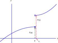
Suppose F is a function defined for all x. We give meaning to the following symbols.
lim F(x) and F’~(a).
Having done so, we ask you to define
lim F(x), and F ,+ (a).
Next we will define limits involving infinity,
lim F(x) and lim F(x) = oo,
x—tco x—*a~
and ask you to define
lim Fix) and lim Fix) = oo.
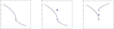
In reading the following two definitions, it will be helpful to study the graphs in Figure 3.27 and assume a = 3.
A
B ‘
Figure 3.27: Graphs of functions F, G, and H that illustrate Definitions 3.7.1 and 3.7.2.
CHAPTER 3. THE DERIVATIVE
171
Definition 3.7.1 Left hand limit and derivative. Suppose F is a function defined for all numbers x except perhaps for a number a and L is a number.
The statement that lim F(x) = L means that
x—*a~
if e is a positive number there is a positive number 5 such that if x is in the domain of F and a — 5 < x < a, then \F(x) — L\ < e.
If F is defined at a, then F’~(a) is defined by
F-(„) = li m f W-f (<0 (3.37)
x^a- x — a
For convenience, in the definitions we have assumed that F is defined for all numbers except perhaps a; in Definition 3.7.1, for example, it would be sufficient to assume that for every number b less than a, the domain of F contains a number between b and a. The condition a — 5 < x < a restricts x to being ‘to the left’ of a (x < a) and within 5 of a. In Figure 3.27A, lim F(x) = 1. In
x— >3~
Figure 3.27C, H’~(3) = —1/3. This may help resolve some dispute as to whether H has a tangent at (3,2) that was mentioned early in this chapter, Explore 3.1.2.
Definition 3.7.2 Limits involving infinity. Suppose F is a function defined for all numbers x except perhaps for a number a and L is a number.
The statement that lim Fix) = L means that if e is a positive number there is a number M so that if x > M, \F(x) — L\ < e. The half-line y = L for x > 0 is said to be a horizontal asymptote of F.
The statement that lim Fix) = oo means that
x^a
if M is a number there is a positive number 5 so that if 0 < \a — x\ < 5, F(x) > M.
In Figure 3.27B, lim G(x) = 2, and lim G(x) does not exist. However, lim G(x) = oo
x >oo x —>3 x —>3~
Explore 3.7.1 Refer to Figure 3.27. For each part below, either evaluate the expression or explain
why it is not denned.
a. lim Fix) b. lim Fix) c. lim Gix)
x^3+ y ‘ x^3 v ‘ x^3+ v ‘
d. F'”(3) e. #’+(3) f. #'(3)
g. lim h. lim i. lim H(x) m
x^oo x^-oo x^-oo
Explore 3.7.2 Write definitions for:
a. lim Fix) — L b. F’ + (a) c. lim Fix) = L
d. lim Fix) = — oo ■
Explore 3.7.3 Attention: Solving this problem may require a significant amount of thought.
We say that lim F{x) exists if either
lim F{x) = —oo, lim F(x) = oo, or for some number L lim F(x) = L.
Is there a function, F, defined for all numbers x such that
lim Fix) does not exist. ■
x-t-l-
Proof of the following theorem is only technical and is omitted.
Theorem 3.7.1 Suppose (p,q) an open interval containing a number a and F is a function defined on (p, q) excepts perhaps at a and L is a number.
lim F(x) = L if and only if both lim F(x) = L and lim F(x) = L. (3.38)
x^a- x^a x^a+
Furthermore, if F is defined at a
F'(a) exists if and only if F’~{a) = F /+ (a), in which case F'(a) = F’~(a). (3.39)
Exercises for Section 3.7 Left and right limits and derivatives; limits involving infinity.
Exercise 3.7.1 For each of the graphs in Figure 3.7.1 of a function, F, answer the questions or assert that there is no answer available.
1. What does Fit) approach as t approaches 3?
2. What does F(t) approach as t approaches 3~?
3. What does F(t) approach as t approaches 3 + ?
4. What is F(3)?
5. Use the limit symbol to express answers to a. – c.
CHAPTER 3. THE DERIVATIVE
Figure for Exercise 3.7.1 Graphs of three functions for Exercise 3.7.1.
173
Exercise 3.7.2 Let functions D, E, F, G, and H be defined by
D(x) = \x\
E(x) =
F(x G(x
x
for all x -1 for x < 0
0 for x = 0
1 for 0 < x
x 2 for x < 0 x for x > 0
1 for x 7^ 0
2 for x = 0
x for x < 0 x 2 for x > 0
A. Sketch the graphs of .D, E, F, G, and i/.
B. Let K be either of D, E, F, G, or H. Evaluate the limits or show that they do not exist.
a. lim K(x)
d. K’-(0)
b. lim K(x)
x— >0+
e.
c. lim K(x)
x^O v ‘
f. K'(0)
Exercise 3.7.3 Define the term ‘tangent from the left’. (We assume you would have a similar definition for ‘tangent from the right’; no need to write it.) What is the relation between tangent from the left, tangent from the right, and tangent?
3.8 Summary of Chapter 3, The Derivative.
You now have an introduction to the concept of rate of change and to the derivative of a function. The derivative and its companion, the integral that is studied in Chapter 9, enabled 10 an explosion in science and mathematics beginning in the late seventeenth century, and remain at the core of science and mathematics today. Briefly, for a suitable function, P, the derivative of P is the function P’ defined by
Pit + h)- P(t)
P'(t)
lim
ft-»o
h
(3.40)
10 It might also be argued that the explosion in science enabled or caused the creation of the derivative and integral. The two are inseparable.
CHAPTER 3. THE DERIVATIVE
174
We also wrote P'(t) as [P(t)}’ and A helpful interpretation of P'(a) is that it is the slope of the tangent to the graph of P at the point (a, P(a)).
The derivatives of three functions were computed (for C a number and n a positive integer) and we wrote what we call primary formulas:
n-l
(3.41)
Two combination formulas were developed:
P(t) = Cu(t)
Pit)
They can also be written
u(t)+v(t) [Cu(t)}’
P’it) = P'(t) =
C [«(*)]’
C x u'(t) u'(t)+v'(t)
(3.42)
We will expand both the list of primary formulas and the list of combination formulas in future chapters and thus expand the array of derivatives that you can compute without explicit reference to the Definition of Derivative Equation 3.40.
We saw that derivatives describe rates of chemical reactions, and used the derivative function to find optimum values of spider web design and the height of a pop fly in baseball. We examined two cases of dynamic systems, mold growth and falling objects, using rates of change rather than the average rates of change used in Chapter 1. A vast array of dynamical systems and optimization problems have been solved since the introduction of calculus. We will see some of them in future chapters.
Finally we defined and computed the second derivative and higher order derivatives and gave some geometric interpretations (concave up and concave down) and some physical interpretation (acceleration).
Exercises for Chapter 3, The Derivative.
Use Definition of t rates of change of the following functions, P.
Chapter Exercise 3.8.1 Use Definition of the Derivative 3.22, lim —to compute the
&-••* b — t
5t 2 c. Pit) = \
2Vi f. Pit) = V2i
5-2* i. Pit) =
5t 7 1. Pit) = %z
CHAPTER 3. THE DERIVATIVE
175
Chapter Exercise 3.8.2 Data from David Dice of Carlton Comprehensive High School in Canada 11 for the decrease in mass of a solution of 1 M HC1 containing chips of CaC0″3 is shown in Table 3.8.0. The reaction is
CaC0 3 (s) + 2HCl(aq) -> C0 2 (g) + H 2 0(1) + CaCl 2 (aq).
The reduction in mass reflects the release of C0 2 .
a. Graph the data.
b. Estimate the rate of change of the mass at each of the times shown.
c. Draw a graph of the rate of change of mass versus the mass.
Table for Exercise 3.8.0 Data for Ex. 3.8.2.
Chapter Exercise 3.8.3 Use derivative formulas 3.41 and 3.42 to compute the derivative of P. Use Primary formulas only in the last step. Assume the t n rule [t n ]’ = nt n ~ x . to be valid for all numbers n, integer, rational, irrational, positive, and negative. In some cases, algebraic simplification will be required before using a derivative formula.
Chapter Exercise 3.8.4 Find an equation of the tangent to the graph of P at the indicated points. Draw the graph P and the tangent.
http: / / www.carlton.paschools.ps.sk.ca/chemical/chem
Chapter 4
Continuity and the Power Chain Rule
Where are we going?
We require the concept of continuity of a function.
The key to understanding continuity is to understand discontinuity. A continuous function is simply a function that has no discontinuity.
The function F whose is graph shown in below is not continuous. It has a discontinuity at the abcissa, a. There are values of x close to a for which F(x) is not close to F(a). F is continuous at all points except a, but F is still said to be discontinuous. In this game, one strike and you are out.
4.1 Continuity.
Most, but not all, of the functions in previous sections and that you will encounter in biology are continuous. Four equivalent definitions of continuity follow, with differing levels of intuition and formality.
Definition 4.1.1 Continuity of a function at a number in its domain.
CHAPTER 4. CONTINUITY AND THE POWER CHAIN RULE
177
Intuitive: A function, f, is continuous at a number a in its domain means that if x is in the domain of f and x is close to a, then f(x) is close to f(a).
Symbolic: A function, f, is continuous at a number a in its domain means that either
or there is an open interval containing a and no other point of the domain of f.
Formal: A function, f, is continuous at a number a in its domain means that for every positive number, e, there is a positive number 5 such that if x is in the domain of f and \x — a\ < 5 then \f(x) – f(a)\ < e.
Geometric A simple graph G is continuous at a point P of G means that if a and (3 are
horizontal lines with P between them there are vertical lines h and k with P between them such that every point of of G between h and k is between a and f3.
Definition 4.1.2 Discontinuous. If a is a number in the domain of a function f at which f is not continuous then f is said to be discontinuous at a.
Definition 4.1.3 Continuous function. A function, f, is continuous means that f is continuous at every number, a, in its domain.
Explore 4.1.1 . Definition 4.1.2 is a sleeper. What does “not continuous” mean? It is a rite of passage for mathematics students to write the negation of the statement that a function is continuous at a number a in its domain. The statement is sometimes called the “logical complement” or the “bare denial” of the statement of continuity at a. To illustrate, the negation of the Symbolic Definition is
Symbolic Definition of Discontinuity: A function, /, which has a number a in its domain is not continuous at a means that every open interval containing a contains a point of the domain of / different from a and either
The Intuitive Definition is so imprecise as to make its negation even more difficult. You should try to write that negation, but will likely first write, “There is a number, x, close to a for which f{x) is not close to f{a),” but this suffers from the uncertainty of “close to.”
Explore 4.1.2 Write the negation of the Formal Definition of Continuity of a function, /, at a point, a, of its domain. This is something into which you can sink your teeth, deeply.
As a guide, we write a negation of the Geometric Definition of continuity.
Geometric Definition of Discontinuity: A simple graph G that contains a point P is not continuous P means that there are horizontal lines a and (3 with P between them such that for any are vertical lines h and k with P between them some point of of G between h and k is not between a and (5. m
Most of the functions that you have experienced are continuous, and to many students it is intuitively obvious from the notation that u(b) approaches u(a) as b approaches a; but in some cases u(b) does not approach u(a) as b approaches a. Some examples demonstrating both continuity and discontinuity follow.
lim/(x) = f(a)

lim f(x) does not exist, or lim f(x) exists and is not = f(a


CHAPTER 4. CONTINUITY AND THE POWER CHAIN RULE
178
Example 4.1.1 1. You showed in Exercise 3.2.7 that every polynomial is continuous.
2. The function describing serum insulin concentration as a function of time is a continuous function even though it may change quickly with serious consequences.
3. The word ‘threshold’ suggests a discontinuous change in one parameter as a related parameter crosses the threshold. Stimulus to neurons causes ion gates to open. When an Na + ion gate is opened, Na + flows into the cell gradually increasing the membrane potential, called a ‘graded response’ (continuous response), up to a certain threshold at which an action potential is triggered (a rapid increase in membrane potential) that appears to be a discontinuous response. As in almost all biological examples, however, the function is actually continuous. See Example Figure 4.1.1.1A.
4. Surprise. The graph in Figure 4.1.1. IB is continuous. There are only three points of the graph. The graph is continuous at, for example, the point (3,2). There is an open interval containing 3, (2.7, 3.3), for example, that contains 3 and no other point of the domain.
Figure for Example 4.1.1.1 A. Events leading to a nerve action potential. B. A discrete
graph is continuous.
A
\2 -50 .O
E
– Stimulus
Action Potential


Threshold
B
Time – milliseconds
( 3 )
5. The function approximating % Female hatched from a clutch of turtle eggs
f 0 if Temp < 28
Percent female = < 50 if Temp = 28 (4.1)
[ 100 if 28 < Temp
is not continuous. The function is discontinuous at t = 28. If the temperature, T, is close to 28 and less than 28, then % Female(T) is 0, which in usual measures is not ‘close to’ 50 = % Female (28).
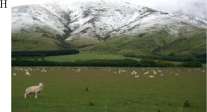
6. As you move up a mountain side, the flora is usually described as being a discontinuous function of altitude. There is a ‘tree line’, below which the dominant plant species are pine and spruce and above which the dominant plant species are low growing brushes and grasses, as illustrated in Figure 4.1.1.1C 1
Figure for Example 4.1.1.1 (Continued.) C. A tree line. Picture taken from the summit of Independence Pass, Colorado at 12,095 feet (3687 m) elevation.
Such a region of apparent discontinuity is termed an ‘ecotone’ by ecologists.
CHAPTER 4. CONTINUITY AND THE POWER CHAIN RULE
179
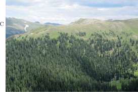
7. We acknowledge that the tree line in Figure 4.1.1.1 is not sharp and some may not agree that it marks a discontinuity.
It is important to the concept of discontinuity that there be an abrupt change in the dependent variable with only a gradual change in the independent variable. Charles Darwin expressed it:
Charles Darwin, Origin of Species. Chap. VI, Difficulties of the Theory. “We see the same fact in ascending mountains, and sometimes it is quite remarkable how abruptly, as Alph. de Candolle has observed, a common alpine species disappears. The same fact has been noticed by E. Forbes in sounding the depths of the sea with the dredge. To those who look at climate and the physical conditions of life as the all-important elements of distribution, these facts ought to cause surprise, as climate and height or depth graduate away insensibly [our emphasis].”
8. From Equation 3.12, lim — = -, the function, f(x) = – is continuous. The graph of fix)
x ^ a x a x certainly changes rapidly near x — 0, and one may think that / is not continuous at x = 0.
However, 0 is not in the domain of f, so that the function is neither continuous nor
discontinuous at x = 0.
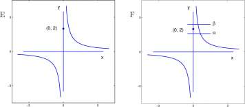
9. Let the function g be defined by
g(x) = – for i/O, g(0) = 2 x
A graph of g is shown in Example Figure 4.1.LIE. The function g is not continuous at 0 and the graph of g is not continuous at (0, 2). Two horizontal lines above and below (0, 2) are drawn in Figure 4.1.1. IF. For every pair of vertical lines h and k with (0, 2) between them there are points of the graph of g between h and k that are not between a and (3.
Figure for Example 4.1.1.1 (Continued) E. The graph of g(x) — 1/x for g(0) = 2.
F. The point (0, 2) and horizontal lines above and below (0, 2).
CHAPTER 4. CONTINUITY AND THE POWER CHAIN RULE
180
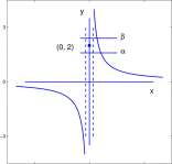
Explore 4.1.3 In Figure 4.1.1 there are two vertical dashed lines with (0,2) between them. It appears that every point of the graph of g between the vertical dashed lines is between the two horizontal lines. Does this contradict the claim made in Item 9? ■
Explore Figure 4.1.1 The graph of g(x) = 1/x for g(0) = 2, horizontal lines above
and below (0,2), and vertical lines (dashed) with (0,2) between them.
-3 0 3
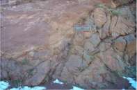
10. The geological age of soil is not a continuous function of depth below the surface. Older soils are at a greater depth, so that the age of soils is (almost always) an increasing function of depth. However, in many locations, soils of some ages are missing: soils of age 400 million years may rest directly on top of soils of age 1.7 billion years as shown in Figure 4.1.1.1. Either soils of the intervening ages were not deposited in that location or they were deposited and subsequently eroded. Geologist speak of an “unconformity” occurring at that location and depth.
Figure for Example 4.1.1.1 (Continued) G. Picture of an unconformity at Red Rocks Park and Amphitheatre near Denver, Colorado. Red 300 million year-old sedimentary rocks rest on gray 1.7 billion year-old metamorphic rocks. (Better picture in “Messages in Stone: Colorado’s Colorful Geology” Vincent Matthews, Katie KellerLynn, and Betty Fox, Colorado Geological Survey, Denver, Colorado, 2003) H. Snow line figure taken in New Zealand for
Exercise 4.1.4.
CHAPTER 4. CONTINUITY AND THE POWER CHAIN RULE
181
11. Every increasing function defined on an interval that is discontinuous at some point has a vertical gap in the graph at that point. Every increasing function with no gap is continuous. Vertical gap: there is a horizontal line that does not intersect the graph, but has a point of the graph below the line and a point of the graph above the line.
Figure for Example 4.1.1.1 (Continued) H. An increasing function. There are two vertical
gaps and two points of discontinuity.
Explore 4.1.4 Vertical gap in the graph G means an interval of the Y-axis that contains no point of the Y-projection of G and for which there is a point of the Y-projection of G below the interval and a point of the Y-projection of G above the interval. Is there a continuous and increasing function that has a vertical gap? ■
H
y = f( t)
Combinations of continuous functions. We showed in Chapter 3 that
lim (Fi(x) + F 2 (x)) = limFi(a;) + lim F 2 (x) Equation 3.14
lim (Fi{x) x F 2 (x))
If lim F 2 (x) + 0, then
limF 1 (x) ) x (limF 2 (x”
lim
F\[x)
lim F\[x)
^ F 2 (x) lim F 2 (x)
Equation 3.15
Equation 3.18
From these results it follows that if u and v are continuous functions with common domain, D, then
u + v
and
u x v
are continuous,
(4.2)
and if v(t) is not zero for any t in D, then
u . A n .
– is continuous. (4.3)
v
Of particular interest is the equation on the limit of composition of two functions,
If lim u(x) = L and lim F(s) = A, then lim F(u(x)) = A, Equation 3.17
X —*ft g —> £j X —
From this it follows that if F and u are continuous and the domain of F contains the range of u then
F o u, the composition of F with u, is continuous. (4.4)
Exercises for Section 4.1, Continuity.
Exercise 4.1.1 1. Find an example of a plant ecotone distinct from the tree line example shown in Figure 4.1.1.1.
2. Find an example of a discontinuity of animal type. Exercise 4.1.2 For f(x) = 1/x,
a. How close must x be to 0.5 in order that f(x) is within 0.01 of 2?
b. How close must a; be to 3 in order to insure that \ be within 0.01 of ^?
c. How close must x be to 0.01 in order to insure that \ be within 0.1 of 100? Exercise 4.1.3 Find the value for u(2) that will make u continuous if
a. u(t) = 2t + 5 for t ^ 2 b. u(t) = for t^2
c. u (t) = for t ^ 2 d – M W = T=\ for t ^ 2
e- u(t) = ^| for t^2 f. u (i)
Exercise 4.1.4 In Example Figure 4.1.1.1 H is a picture of snow that fell on the side of a mountain the night before the picture was taken. There is a ‘snow line’, a horizontal separation of the snow from terrain free of snow below the line. ‘Snow’ is a discontinuous function of altitude. Explain the source of the discontinuity.
Exercise 4.1.5 a. Draw the graph of y\. b. Find a number A such that the graph of y 2 is continuous.
a. y x {x)
x 2 for x < 2 x 2 for x < 2
b. y 2 (x) = <
3 — x for 2 < x A — x for 2 < rr
CHAPTER 4. CONTINUITY AND THE POWER CHAIN RULE
183
Exercise 4.1.6 Is the temperature of the water in a lake a continuous function of depth? Write a paragraph discussing water temperature as a function of depth in a lake and how knowledge of water temperature assists in the location of fish.
Exercise 4.1.7 To reduce inflammation in a shoulder, a doctor prescribes that twice daily one Voltaren tablet (25 mg) to be taken with food. Draw a graph representative of the amount of Voltaren in the body as a function of time for a one week period. Is your graph continuous?
Exercise 4.1.8 The function, f(x) = ifx is continuous.
1. How close must x be to 1 in order to insure that f(x) is within 0.1 of /(l) = 1 (that is, to
insure that 0.9 < f(x) < 1.1)?
2. How close must x be to 1/8 in order to insure that f(x) is within 0.0001 of /(1/8) = 1/2 (that is, to insure that 0.4999 < f(x) < 0.5001)?
3. How close must a; be to 0 in order to insure that f(x) is within 0.1 of /(0) = 0?
b. Does your graph intersect the X-axis?
c. Draw a graph of of a function, /, defined on the interval [1, 3] such that /(l) = —2 and /(3) = 4 that does not intersect the X-axis. Be sure that its X-projection is all of [1, 3].
d. Write equations to define a function, /, on the interval [1, 3] such that /(l) = —2 and /(3) = 4 and the graph of / does not intersect the X-axis.
e. There is a theorem that asserts that the function you just defined must be discontinuous at some number in [1,3]. Identify such a number for your example.
The preceding exercise illustrates a general property of continuous functions called the intermediate value property. Briefly it says that a continuous function defined on an interval that has both positive and negative values on the interval, must also be zero somewhere on the interval. In language of graphs, the graph of a continuous function defined on an interval that has a point below the X-axis and a point above the X-axis must intersect the X-axis. The proof of this property requires more than the familiar properties of addition, multiplication, and order of the real numbers. It requires the completion property of the real numbers, Axiom 5.2.1 2 .
Exercise 4.1.10 A nutritionist studying plasma epinephrine (EPI) kinetics with tritium labeled epinephrine, [ 3 H]EPI, observes that after a bolus injection of [ 3 H]EPI into plasma, the time-dependence of [ 3 H]EPI level is well approximated by L(t) = 4e~ 2t + 3e~* where L(t) is the level of [ 3 H]EPI t hours after infusion. Sketch the graph of L. Observe that L(0) = 7 and L(2) = 0.479268. The intermediate value property asserts that at some time between 0 and 2 hours the level of [ 3 H]EPI will be 1.0. At what time, t u will L(ti) = 1.0? (Let A = e * and observe that
Exercise 4.1.9
/(1) = –
9 a. Draw the graph of a function, /, defined on the interval [1, 3] such that 2 and /(3) = 4.
A 2 =

2 The intermediate value property is equivalent to the completion property within the usual axioms of the number system. See Exercise 12.1.8
CHAPTER 4. CONTINUITY AND THE POWER CHAIN RULE
184
Exercise 4.1.11 For the function, f(x) = 10 — x 2 , find an an open interval, (3 — 5,3 + 5) so that f(x) > 0 for a; in (3-5,3 + 5).
Exercise 4.1.12 For the function, f(x) = sin(x), find an an open interval, (3 — 5,3 + 5) so that f(x) > 0 for a; in (3-5,3 + 5).
Exercise 4.1.13 The previous two problems illustrate a property of continuous functions formulated in the Locally Positive Theorem:
Theorem 4.1.1 Locally Positive Theorem. If a function, f, is continuous at a number a in its domain and f(a) is positive, then there is a positive number, 5, such that f(x) is positive for every number x in (a — 5, a + 5) and in the domain of f.
Prove the Locally Positive Theorem. Your proof may begin:
1. Suppose the hypothesis of the Locally Positive Theorem.
2. Let e = f(a).
3. Use the hypothesis that lim^a f(x) = f(a).
Exercise 4.1.14 Is it true that if a function, /, is positive at a number a in its domain, then there is a positive number, 5, such that if x is in (a — 5, a + 5) and in the domain of / then f(x) > 0?
4.2 The Derivative Requires Continuity.
Suppose u is a function.
u i 0 \ _ 5
If lim = 4, what is lim u(b) ?
6->3 b-3 £>->3 V ‘
The answer is that
We reason that
lim u(b) = 5
6—>3
u ( 0 \ _ 5
for b close to 3, the numerator of — is close to 4 times the denominator.
6-3
That is, u(b) – 5 is close to Ax (b-3).
But 4 x (b — 3) is also close to zero. Therefore If b is close to 3, u(b) — 5 is close to zero and u(b) is close to 5. The general question we address is:
Theorem 4.2.1 The Derivative Requires Continuity. If u is a function and u'(t) exists at t — a then u is continuous at t — a.
CHAPTER 4. CONTINUITY AND THE POWER CHAIN RULE
185
Proof. In Exercise 4.2.2 you are asked to give reasons for the following steps, (i) Suppose the hypothesis of Theorem 4.2.1.
– (v
(lim u(b)
u\a)
lim (u(b) — u(a)) . u{b)-u{a)
(0
lim
b^a b — a
u(b) — u(a)
lim
b^a
x (b — a)
x lim (b — a)
b – a b->a
u'(a) lim (6 — a)
b^a
lim u(b)
b—>a
End of proof.
A graph of a function u defined by
ill a,)
(ii) (Hi) (iv) (v)
(4.5)
u(t)
0 for 20 < t < 28
50 for t = 28
100 for 28 < t < 30
(4.6)
is shown in Figure 4.1A. We observed in Section 4.1 that u is not continuous at t — 28.
( lim u(t) = 0 7^ 50 = m(28).) Furthermore, w'(28) does not exist. A secant to the graph through
t —>28 —
(6, 0) and (28, 50) with b < 28 is drawn in Figure 4.IB, and
u(b) – u{28) 0-50
for b < 28,
50
6- 28 6- 28 28 -6
The slope of the secant gets greater and greater as 6 gets close to 28.
A
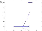
Figure 4.1: A. Graph of The function u defined in Equation 4.6. B. Graph of u and a secant to the graph through (6,0) and (28,50).
Explore 4.2.1 Is there a line tangent to the graph of u shown in Figure 4.1 at the point (28,50) of the graph? ■
CHAPTER 4. CONTINUITY AND THE POWER CHAIN RULE
186
A
(0,0)
B
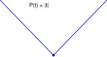
Figure 4.2: a. Graph of P(t) = \t\ for all t. B. Graph of (P(t) – P(0))/(i – 0).
Explore 4.2.2 In Explore Figure 4.2.2 is the graph of y = J\x\. Does the graph have a tangent at (0,0)? Your vote counts. ■
Explore Figure 4.2.2 Graph of y = J\x\.
The graph of P(t) = \t\ for all t is shown in Figure 4.2A. P is continuous, but P'(0) does not
exist.
P(b) – P(0) _ [6|-0 _ |6| _ f -1 for b < 0 6 – 0 6-0 ~ b ~ | 1 for b > 0
A graph of —^-t —is shown in Figure 4.2B. It should be clear that
6-0
Mm f <“> – P <°> fc^o 6-0
does not exist, so that P'(0) does not exist.
Therefore, the converse of Theorem 4.2.1 is not true. Continuity does not imply that the derivative exists.
Exercises for Section 4.2, The Derivative Requires Continuity.
Exercise 4.2.1 Shown in Figure 4.2.1 is the graph of C(t) = \fi.
a. Use Definition of Derivative Equation 3.22 to show that C”(0) does not exist.
b. Is C(t) continuous?
c. Is there a line tangent to the graph of C at (0,0)?
Figure for Exercise 4.2.1 Graph of C(t) — \/i for Exercise 4.2.1.
-2-1 0 1 2
Exercise 4.2.2 Justify the steps (i) — (v) in Equations 4.5.
Exercise 4.2.3 For for the function P(t) = \t\ for all t compute P’~(0) and P /+ (0).
Explore 4.2.3 This problem may require extensive thought. Is there a function defined for all numbers t and continuous at every number t and for which / /_ (1) does not exist? ■
4.3 The generalized power rule.
In Section 3.5 we proved the Power Rule: for all positive integers, n,
[t n ]’ = nt n ~ 1 We show here the generalized power rule.
Suppose n is a positive integer and u(t) is a function that has a derivative for all t. We use the notation
(u(t)) n = u n (t). Then \u n (t)}’ = nu n ^(t) x u'(t). (4.7)
The generalized power rule is used in the following setting. Suppose
P(t) = (l + t 2 ) 3
There are two options for computing P'(t). Option A. Expand the binomial:
Pit) = (l + t 2 ) 3
= l + 3t 2 + 3t 4 + t 6
CHAPTER 4. CONTINUITY AND THE POWER CHAIN RULE
188
Then use the Sum, Constant, Constant Factor, and Power Rules to show that
P'{t) = 0 + Qt + 12t 3 + Qt 5 Option B. Use the Generalized Power Rule with u(t) = 1 + t 2 . Then
P(t) = (1 + t 2 ) 3 P'(t) = 3(1+ t 2 ) 2 x [1 + t 2 ]’
3 (1 + t 2 f x 2t
= « 3 (*)
= 3u 2 (t) x u'(t)
The answers are the same, for
3 ( 1 + t 2 Y x 2t = 3 ( 1 + 2t 2 + t 4 ) x 2t = 6t + 12t 3 + 6t 5
Option A (expand the binomial) may appear easier than Option B (use the generalized power rule), but the generalized power rule is clearly easier for a problem like
Compute P'{t) for P(t) = ( 1 + t 2 )
10
Expanding (1 + 1 2 ) 10 into polynomial form is tedious (if you try it you may conclude that it is a worse than tedious). On the other hand, using the generalize power rule
p\t) = io (i + t 2 ) !
x
i + r
‘ = 10 (l + t 2 ) 9 x 2t
A special strength of the generalized power rule is that when u is positive, Equation 4.7 is valid for all numbers n (integer, rational, irrational, positive, negative). Thus for P(t) = \J\ + 1 2 ,
P\t) =
(i + t 2 y
Change to fractional exponent.
= \( 1 + t 2 ) 3 1 x [ 1 + t 2 }’ Generalized Power Rule.
= \ (1 + t 2 y^ x 2t Sum, Constant, Power Rules
You will prove that when u is positive Equation 4.7, [u n {t]}’ = nu n ~ l x u'(t), is valid for n a negative integer (Exercise 4.3.3) and for n a rational number (Exercise 4.3.4).
Proof of the Generalized Power Rule. Assume that n is a positive integer, u(t) is a function and u'{t) exists. Then
Equations to prove the GPR. See Exercise 4.3.2.
(4.8)
CHAPTER 4. CONTINUITY AND THE POWER CHAIN RULE
189
[u n (t)}’ = lim
u n (b) – u n (t)
lim
b^t
b-*t b-t
u n ~\b) + u n ~ 2 {b) u(t) + ■■■ + u(b) u n ~ 2 {t) + « n_1 (t)) x (u(b) – u(t))
b-t
lim ^(u n -\b) + u n 2 {b) u{t) + ■■■ + u{b) u n ‘ 2 (t) + ^(t))
(«(6) – u(t) b-t
lim (« n_1 (6) + u n 2 (b) u(t) + ■■■ + u(b) u n 2 (t) + « n_1 (t)) x lim ( M ( 6 ) _ “(*))
lim (u n_1 (&) + « n 2 (6) u(t) + • • • + u(6) u n ~ 2 (i) + « n_1 (t)) x u'(i)
(lim u n 1 (6) + lim u n 2 (fe)u(t) + • • • + lim «(6) u”2 (t) + lim u” -1 ^ x «'(t)
\b—*t b—*t b—*t b—*t )
lim u n ~\b) + u(i) lim u n ~ 2 (6) + • • • + u n ” 2 (t) lim + lim u n ~\t) x
b^t b—*t b—*t b—*t )
lim u”” 1 ^) + u(t) lim u n ~ 2 (b) +■■■ + u n ~ 2 {t) lim u(6) + u n ~ l {t)] x u'(t)
b^t b—*t )
lim u n_1 (6) + u(t) lim u”~ 2 (6) + • • • + u n ~ 2 {t) lim xn(t) + u””^*)”) x u'(t)
b—*t b—*t b—*t )
VI)
vii)
viii)
ix)
u n L (t)+u n -\t) + — + u n -\t) + u n L (t)\ xu'{t) (.r) n terms
= nu n -\t) x u'{t) Whew! End of Proof.
Explore 4.3.1 In Explore Figure 4.3.1 is a graph of F defined by
F(x) = x for x = 0 or x is the reciprocal of a positive integer.
Only 13 of the infinitely many points of the graph of F are plotted. What is the graph of F’7 Your vote counts. ■
0
III)
CHAPTER 4. CONTINUITY AND THE POWER CHAIN RULE
190
Explore Figure 4.3.1 Thirteen of the infinitely many points of the graph of y = x for x = 0 or x is the reciprocal of a positive integer.
o- •
0 0.2 0.4 0.6 O.E
To demonstrate use of the generalized power rule, we announce a Primary Formula that is proved in Chapter 7.
[ sin t ]’ = cost, (4.9)
The derivative of the sine function is the cosine function. Then, for (sint) 2 = sin 2 t,
= 2sin 2_1 t x [sint]’ Generalized Power Rule
= 2 sint x cost Equation 4.9
Now consider that cost = y/Y — sin 2 t for 0 < t < it/ 2.
sin 2 t
[cos t)’
1 – sin 2 1 A 5
sin 2 tY x
1 – sin 2 1
I(l-sin 2 t) 5 x [11′
sin 2 1
Definition of P Generalized Power Rule Sum Rule for Derivatives
(4.10)
1
x 0 — 2 sin t cos t
1 – sin 2 1
[C]’ = 0 and Eq 4.10
= — sin t Trigonometric simplification.
One might then guess (correctly) that
[cost]’ = — sin t for all t.
Observe the exaggerated I J’s in the step marked ‘Sum Rule for Derivatives.’ Students tend to omit writing those parentheses. They may carry them mentally or may loose them. The ( )’s are
CHAPTER 4. CONTINUITY AND THE POWER CHAIN RULE
191
necessary. Without them, the steps would lead to
P> = ^(l-sin 2 *) 1 1
= Kl-sin^^xfl]’
1 – sin 2 t
sin 2 t
= —2 sin t cos t Unfortunately, the answer is incorrect. Always:
Generalized Power Rule
Sum Rule for Derivatives
= | (l – sin 2 t)” 1 x 0 – 2sintcost [ C]’ = 0 and Eq 4.10
Trigonometric simplification.
First Notice. Use parentheses, ( )’s, they are cheap.
4.3.1 The Power Chain Rule.
The Generalized Power Rule is one of a collection of rules called chain rules and henceforth we will refer to it as the Power Chain Rule. The reason for the word, ‘chain’ is that the rule is often a ‘link’ in a ‘chain’ of steps leading to a derivative. Because of its form
[u(t) n ]’ = nu(t) n 1 x [«(*)]’,
when the Power Chain Rule is used, there always remains a derivative, [u(t) ] , to compute after the Power Chain Rule is used. The power chain rule is never the final step — the final step is always one or more of the Primary Formulas.
For example, compute the derivative of
= — 1 ^ = (i + (x+if 2 Y 1
y =
= (-1) (l + (x + if 2 )’ 2 X [l + (x +
= (-1) (i + (x+i) i/2 y 2 (o+[(x+ i) 1 / 2 ]’)
= (-1) (l + (x + if 2 )” (l/2)(x + l)1 / 2 [x + 1}’
= (-1) (l + (x + if 2 )” (l/2)(x + 1)-V2(i + o)
Logical Identity
Power Chain Rule
Sum and Constant Rules
Power Chain Rule
Power and Constant Rules
CHAPTER 4. CONTINUITY AND THE POWER CHAIN RULE
192
Exercises for Section 4.3, The generalized power rule. Exercise 4.3.1 Compute P'(t) for
1 + sint) 3
(6t 7 + 5 4 ) 9 (t 2 + sint) 13
(i + i) 2
2
(i + t y
Exercise 4.3.2 Give reasons to support each of the equality signs labeled (i) — quad — (x) in Equations 4.8 to prove the Generalized Power Rule. Each equality can be justified by reference to algebra, to one of the limit formulas Equations 3.10 through 3.15 (shown next), or Theorem 4.2.1, The Derivative Requires Continuity, or the definition of the derivative, Equation 3.22. Equations 3.10 through 3.15 are:
Eq 3.10 lim C = C Eq 3.11 lim x = a
x^a x^a
Eq3.12 lim – = – Eq 3.13 lim C Fix) = C lim Fix)
x—>a jr a ‘ x^a x~^a
Eq 3.14 lim iFAx) + F 2 (x)) = lim FAx) + lim F 2 (x)
x—>a x—*a x~*a
Eq3.15 lim (F^x) x F 2 (x)) = ( lim F^x)) x (lim F 2 (x)) Eq 3.22 F’ix) = lim F ^ – F ^
b^x b – X
Exercise 4.3.3 Suppose m is a positive integer and a function u has a derivative at t and that u(t) 7^ 0. Give reasons for the equalities (i) — (vii) below that show
u m {t)}’ = (-m) u~ m ~^it) x u'(t)
CHAPTER 4. CONTINUITY AND THE POWER CHAIN RULE
193
\u~ m {t)] v =’ lim
(1) ls _ «-“*(&) – u”™(t)
6^0 6 — t
1 1
= lim
u m {b) u m {t)
b-*t b-t
, u m m – u m (6) 1 lim – ^4 x
6-t u m (b) x u m (i) 6 – t
x lim
b-t
u(b) – u(t)
b->t b-t
x hm —^ —
6-t-t 0 — t
(«») + tt 1 “-^) + • • • u^jt) + ir-^m
X tl'(t)
(vii)
u m (t) x w m (t) (-m) um -\t) x «'(*)
X ti'(t)
Exercise 4.3.4 Suppose p and q are integers and w is a positive function that has a derivative at
all numbers t. Assume that
u*(t) exists. Give reasons for the steps (i) — (iv ) below that show u«(t)
jju< -1 (t) x u'{t).
Let Then
= u«(t). v i(t) = u p (t)
gu 5_1 (t) x = puP-^t) x «'(*)
u?(t)
2u5 _1 (i) x u'(i)
(0
(«)
(in) (iu)
CHAPTER 4. CONTINUITY AND THE POWER CHAIN RULE
194
4.4 Applications of the Power Chain Rule.
The Power Chain Rule
PCR: [u n (t)f = nu n -\t) x u'(t) = n u 11 ‘ 1 (t) u (t) (4.11)
greatly expands the diversity and interest of problems that we can analyze. Note that the second form omits the x symbol; multiplication is implied by the juxtaposition of symbols. The general chain rule also will be written
[ G(u(x))}’ = G'{u{x))u'{x) Some introductory examples follow.
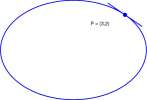
Example 4.4.1 A. Find the slope of the tangent to the circle, x 2 + y 2 = 13, at the point (2,3). See Figure 4.3.
B. Also find the slope of the tangent to the circle, x 2 + y 2 = 13, at the point (3,-2).
Figure 4.3: Graph of the circle x 2 +y 2 = 13 and tangents drawn at the points (2,3) and (3,-2) of the circle.
Solution First check that 2 2 + 3 2 = 4 + 9 = 13, so that (2,3) is indeed a point of the circle. Then solve for y in x 2 + y 2 = 13 to get
CHAPTER 4. CONTINUITY AND THE POWER CHAIN RULE
Then the Power Chain Rule with n =\ yields
V13 –
i3-x 2 y
(i) Symbolic identity
= | (13 – x 2 )^ x [ 13 – x 2 }’ (ii) PCR, n = 1/2 u = 1 – x 2
= 1(13-x 2 y^ x ^[13]’- [x 2 ]’^j (iii) Sum Rule
= |(13-x 2 )~ 5 x^0-2a;^ (w) Constant and Power Rules
= — x
(13-:r 2 H
Observe the exaggerated y J’s in steps (iii) and (iv). Students tend to omit writing them, but they are necessary. Without the ( )’s, steps (iii) and (iv) would lead to
y [ = l(i3-x 2 y^ x [13]’ -[x 2 ^
= 1(13 -x 2 Y^ x 0 -2x = -2x
(iii) Sum Rule
(iv) Constant and Power Rules
a notably simpler answer, but unfortunately incorrect. Always:
Second Notice. Use parentheses, ( )’s, they are cheap.
To finish the computation, we compute y[ at x = 2 and get
I/i(2) = (-2) (l3-2 2 )^ = -^
and the slope of the tangent to x 2 + y 2 = 13 at (2,3) is -2/3. An equation of the tangent is
y-3 2 2 1
= — or y = — x + 4-
x-2 3 y 3 3
B. Now we find the tangent to the circle x 2 + y 2 = 13 at the point (3,-2). Observe that 3 2 + (-2) 2 = 4 + 9 = 13 so that (2,-3) is a point of x 2 + y 2 = 13, but (3,-2) does not satisfy
because
yi = (l3-x 2 Y -2 ^ (13- (-3)2 2 )’ =2
CHAPTER 4. CONTINUITY AND THE POWER CHAIN RULE
196
For (3,-2) we must use the lower semicircle and
y 2 = -(l3-X 2 y
Then
y 2
(l3-x 2 )
2 \ 2
1 – x z
-2x)
At x = 3
y’ 2 (3) =
1 (13-3 2 ) § (-2×3) = 3
2 v / ” ‘2
and the slope of the line drawn is 3/2. m
It is often helpful to put the denominator of a fraction into the numerator with a negative exponent. For example:
Problem. Compute P'(t) for P(t)
P’it) –
+ 0
2 •
Solution
= 5
(1 + t) 2 5(1 + t)2
5((-2)(i+tr 3 ) x [(i+or
= 5 (-2) (1 + t)’ 3 x 1 = -10 (l + ty 3 aaa We will find additional important uses of the power rules in the next section.
Exercises for Section 4.4, Applications of the Power Chain Rule. Exercise 4.4.1 Compute y'(x) for
a. y — 2x 3 – 5
d. y = (l + x 2 ) 0 5 g. y = (2-xf
m.
b. y =
2
x 2
= VT
x c
e. y h. y = (3-x 2 ) 4
c. y =
(x + 1) 2
f. y = (l-x 2 )0 5
l. y =
x/
j. y = (l + (x-2) 2 ) z k. y = (l + 3x) Lb 1. y =
Vl6 –
CHAPTER 4. CONTINUITY AND THE POWER CHAIN RULE 197 Exercise 4.4.2 Shown in Figure Ex. 4.4.2 is the ellipse,
2 2
x y
— + — = 1
18 8
and a tangent to the ellipse at (3,2).
a. Find the slope of the tangent.
b. Find an equation of the tangent.
c. Find the x- and ^/-intercepts of the tangent.
Figure for Exercise 4.4.2 Graph of the ellipse x 2 /18 + y 2 /8 = 1 and a tangent to the ellipse at
the point (3,2).
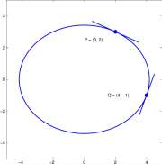
Exercise 4.4.3 Shown Figure Ex. 4.4.3 is the ellipse,
2x 2 3y 2
+ — = 1
35 35
and tangents to the ellipse at (2, 3) and at (4, -1).
a. Find the slopes of the tangents.
b. Find equations of the tangents.
c. Find the point of intersection of the tangents.
Figure for Exercise 4.4.3 Graph of the ellipse 2x 2 /35 + 3y 2 /35 = 1 and tangents to the ellipse
at the points (2,3) and (4,-1).
CHAPTER 4. CONTINUITY AND THE POWER CHAIN RULE
198
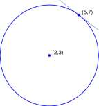
Exercise 4.4.4 Shown in Figure Ex. 4.4.4 is the circle with center at (2,3) and radius 5. find the slope of the tangent to this circle at the point (5,7). An equation of the circle is
(x – 2) 2 + (y – 3) 2 = 5 2
Figure for Exercise 4.4.4 Graph of the circle (x — 2) 2 + (y — 3) 2 = 5 2 and tangent to the circle
at the point (5,7).
4.5 Some optimization problems.
In Section 3.5.2 we found that local maxima and minima are often points at which the derivative is zero. The algebraic functions for which we can now compute derivatives have only a finite number of points at which the derivative is zero or does not exist and it is usually a simple matter to search among them for the highest or lowest points of their graphs. Such a process has long been used to find optimum parameter values and a few of the traditional problems that can be solved using the derivative rules of this chapter are included here. More optimization problems appear in Chapter 8 Applications of the Derivative.
Assume for this section only that all local maxima and local minima of a function, F, are found by computing F’ and solving for x in F'(x) = 0.
CHAPTER 4. CONTINUITY AND THE POWER CHAIN RULE
199
Example 4.5.1 A forester needs to get from point A on a road to point B in a forest (see diagram in Figure 4.4). She can travel 5 km/hr on the road and 3 km/hr in the forest. At what point, P, should she leave the road and enter the forest in order to minimize the time required to travel from A to B7
<-
6 km
Road
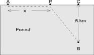
Figure 4.4: Diagram of a forest and adjacent road for Example 4.5.1
Solution. She might go directly from A to B through the forest; she might travel from A to C and then to B; or she might, as illustrated by the dashed line, travel from A to a point, P, along the road and then from P to B.
Assume that the road is straight, the distance from B to the road is 5 km and the distance from A to the projection of B onto the road (point Q) is 6 km. The point, P, is where the forester leaves the road; let x be the distance from A to P. The basic relation between distance, speed, and time is that
Distance (km) = Speed (km/hr) x Time (hr)
so that
Distance Speed
The distance traveled and time required are
Along the road In the forest
Distance x
Time j£ (
The total trip time, T, is written as
T =l + — ^ ( 4 12 )
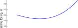
A graph of T vs x is shown in Figure 4.5. It appears that the lowest point on the curve occurs at about x = 2.5 km and T = 2.5 hours. H
CHAPTER 4. CONTINUITY AND THE POWER CHAIN RULE
200
2 9 –
*~ 2.3 –
2 I 1 1 1 1 1 1 1 1
-1 01234567
x – Distance AP, km
Figure 4.5: Graph of Equation 4.12; total trip time, T, vs distance traveled along the road, x before entering the forest.
Explore 4.5.1 It appears that to minimize the time of the trip, the forester should travel about 2.5 km along the road from A to a point P and enter the forest to travel to B. Observe that the tangent to the graph at the lowest point is horizontal, and that no other point of the graph has a horizontal tangent.
Compute the derivative of T(x) for
T(x)
x J{6 – x y
5 3
Note: The constant denominators may be factored out, as in
1
X 1
You should get
T'{x)
1 1
32
(Q-x) 2 + 5 2 ) x2(6-x)(-l)
Find the value of x for which T'(x) = 0.
Your conclusion should be that the forester should travel 2.25 km from A to P and that the time for the trip, T(2.25) = 2.533 hours. ■
Exercises for Section 4.5, Some optimization problems.
Exercise 4.5.1 In Example 4.5.1, what should be the path of the forester if she can travel lOkm/hr on the road and 4km/hr in the forest?
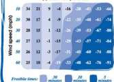
Exercise 4.5.2 The air temperature is -10° F and Linda has a ten mile bicycle ride from the university to her home. There is no wind blowing, but riding her bicycle increases the effects of the cold, according to the wind chill chart in Figure 4.5.2 provided by the Centers for Disease Control. The formula for computing windchill is
CHAPTER 4. CONTINUITY AND THE POWER CHAIN RULE
201
where: T = Air Temperature (F) and V = Wind Speed (mph).
Assume that if she travels at a speed, s, then she looses body heat a rate proportional to the difference between her body temperature and wind chill temperature for speed s. (Because no wind is blowing, V — s).
a. At what speed should she travel in order to minimize the amount of body heat that she looses during the 10 mile bicycle ride?
b. Frostbite is skin tissue damage caused by prolonged skin tissue temperature of 23°F. The time for frostbite to occur is also shown in Figure 4.5.2. What is her optimum speed if she wishes to avoid frostbite.
c. Discuss her options if the ambient air temperature is -20°F.
Figure for Exercise 4.5.2 Table of windchill temperatures for values of ambient air temperatures and wind speeds provided by the Center for Disease Control at http://emergency.cdc.gov/disasters/w...cold_guide.pdf. It was adapted from a more detailed chart at http://www.nws.noaa.gov/om/windchill.
Wind Chill Factor
Actuot olf temperature *F
Apparent temperature ■4
f
m\nutri
Exercise 4.5.3 If x pounds per acre of nitrogen fertilizer are spread on a corn field, the yield is
200 4000
x + 25
bushels per acre. Corn is worth $6.50 per bushel and nitrogen costs $0.63 per pound. All other costs of growing and harvesting the crop amount to $760 per acre, and are independent of the amount of nitrogen fertilizer applied. How much nitrogen per acre should be used to maximize the net dollar return per acre? Note: The parameters of this problem are difficult to keep up to date.
Exercise 4.5.4 Optimum cross section of your femur. R. M. Alexander 3 has an interesting analysis of the cross section of mammal femurs. Femurs are hollow tubes filled with marrow. They should resist forces that tend to bend them, but not be so massive as to impair movement. An
CHAPTER 4. CONTINUITY AND THE POWER CHAIN RULE
202
optimum femur will be the lightest bone that is strong enough to resist the maximum bending moment, M, that will be applied to it during the life of the animal.
A hollow tube of mass m kg/m may be stronger than a solid rod of the same weight, depending on two parameters of the tube, the outside radius, R, and the inside radius, x x R (0 < x < 1), see Figure 4.6. For a given moment, M, the relation between R and x is
R =
M
K(l-x 4
k) (1
4\-±
1 3
* 4 )
(4.13)
The constant K describes the strength of the material.
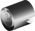
Figure 4.6: Consider a femur to be a tube of radius R with solid bone between kR and R and marrow inside the tube of radius kR.
Let p be bone density and assume marrow density is \p. Then the mass per unit length of bone, nib, is
m b = p x (ttR 2 – ir(R x x) 2 )
= pn(l-x 2 )R 2
(4.14)
= pn(fY -*<)-§
a. Write an equation for the mass per unit length of the bone marrow similar to Equation 4.14.
b. Let m be total mass per unit length; the sum of m& and the mass per unit length of marrow. We would like to know the derivative of m with respect to x for
m = c((l–x 2 ) (l-x 4 )-§). C = piv(
K
(4.15)
You will see in Chapter 6 that
[m]’ = C
1 – -x l
x (l-x 4 )-I + (1- \x 2 ) x Ul-x 4 )-! 1 ‘
Finish the computation of [m]’ and simplify the expression.
CHAPTER 4. CONTINUITY AND THE POWER CHAIN RULE
203
c. Find a value of x for which x = x yields m! = 0.
-x(l-x 4 ) _i + ^ 3 (l-^ 2 ) (l-a; 4 )” § =0
d. The value x computed in Part c. is the x-coordinate of the lowest point of the graph of m shown in Exercise Figure 4.5.4. Alexander shows the values for x for five mammalian species; for the humerus they range from 0.42 to 0.66 and for the femur they range from 0.54 to 0.63. Compare x with these values.
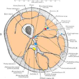
e. Exercise Figure 4.5.4B is a cross section of the human leg at mid-thigh. Estimate x for the femur.
Alexander modifies this result, noting that Equation 4.13 is the breaking moment, and a bone with walls this thin would buckle before it broke, and noting that bones are tapered rather than of uniform width.
Figure for Exercise 4.5.4
CHAPTER 4. CONTINUITY AND THE POWER CHAIN RULE
204
A. Graph of Equation 4.15, m, the mass of bone plus marrow, as a function of the ratio, x. Mass per unit length of a solid bone has been arbitrarily set equal to one. B. Cross section of a human leg at mid thigh, http://en.wikipedia.org/wiki/Fascial...ments_of_thigh. Lithograph plate from Gray’s Anatomy, not copyrightable.
A. 1
4.6 Implicit differentiation.
In Section 4.4, Applications of the Power Chain Rule, we found slopes of circles and ellipses. There is a procedure for finding these slopes that requires less algebra, but more mathematical sophistication. In each of the equations,
CHAPTER 4. CONTINUITY AND THE POWER CHAIN RULE
205
18 8
2 x 2 3y 2
+ — = 1
35 35
we might solve for y in terms of x, being careful to choose the correct square root to match the point of tangency, and then compute y'(x).
In x 2 + y 2 = 13, we may chose y(x) = Vl3 — x 2 . Note that
x 2 + y 2 = x 2 + (Vl3-x 2 ) 2 = x 2 + 13 – = 13
so that y(x) = y/13 — x 2 is a function that ‘satisfies’ and is said to be implicitly defined by the equation.
Definition 4.6.1 Implicit Function. Suppose we are given an equation
E(x,y) = 0
and point (a, b) for which
E(a,b) = 0
A function, f, defined on an interval (a — h,a + h) surrounding a and satisfying
E(xj(x)) = 0 and f(a) = b
is said to be implicitly defined by E. There may be no such function, f, one such function, or many such functions.
Now we assume without solving for y(x) that there is a function y(x) for which
x 2 + {y{x)f = 13 and y(2) = 3, and use the power rule and power chain rule to differentiate the terms in the equation, as follows.
x 2 + (y(x)) 2 = 13
x
+
y(x)) 2 }’ = [13]’
2 x + 2 y(x) y'{x) = 0
The power rule is used for
The power chain rule is used for
x
= 2x
y{x)
2y(x) y'{x)
CHAPTER 4. CONTINUITY AND THE POWER CHAIN RULE
206
We use x = 2 and y{2) = 3 in the last equation to get
2×2 + 2×3 y'{2) = 0
and solve for y'(2) to get
,'(2) = -I
as was found in Example 4.4.1 to be the slope of the tangent to x 2 + y 2 = 13 at (2,3).
It is important to remember in the above steps the [ ]’ means derivative with respect to the independent variable, x. The Leibnitz notation, explicitly shows this and may be easier to use. We repeat this problem with Leibnitz notation.
x 2 + (y(x)f = 13 2x + 2y(x)-^y(x) = 0
The power rule is used for The power chain rule is used for
i( x2 ) =2x Tx {y{x))2 = 2y{x) Tx y{x)
Example 4.6.1 We consider another example of implicit differentiation. Find the slope of the graph of
y/x + \/5-y 2 = 5 at (9,1) and at (4,2) First we check to see that (9,1) satisfies the equation:
V9 + Vb^l 2 = V9 + 41 = 3 + 2 = 5. It checks. Then we assume there is a function y(x) such that
y/x + \Jh – (y(x)) 2 = 5 and that y(9) = 1. We convert the square root symbols to fractional exponents and differentiate using Leibnitz
CHAPTER 4. CONTINUITY AND THE POWER CHAIN RULE
207
notation.
\x 2 + | (5 — y 2 ) 2 (o — 2y-^y(x)^j = 0 Constant and Power Chain Rules
Next we solve for £y(x) and get
d_ dx
y(x)
2yx 7 <
and evaluate at (9,1)
2yx 7 <
(x,y)=(9,l)
1
3
So the slope of the graph at (9,1) is 1/3. You may notice that we have selectively used y(x) and y; often only y is used to simplify notation.
An equation of the tangent to the graph of ^fx + 5 — y 2 = 5 at the point (9,1) is
Now for the point (4,2), the differentiation is exactly the same and we might (alert!) evaluate
d
dx
y(x)
5-y 2
2yx l
at (4,2)
5-yi
2yx^
(x,y)=(4,2)
1
8
However, the point (4,2) does not satisfy the original equation and is not a point of its graph. Finding the slope at that point is meaningless, so we punt.
All of this solution is algebraic. The graph of the equation shown in Figure 4.7 is of considerable help, h
Exercises for Section 4.6 Implicit Differentiation.
Exercise 4.6.1 For those points that are on the graph, find the slopes of the tangents to the graph of
2 2
a. + ^- = 1 at the points (3,2) and (-3,2)
b. ^ + ^ = 1 at the points (4,1), (-3,-2), and (4,-1)
Exercise 4.6.2 Find the slope of the graph of ^fx — ^5 — y 2 = 5 at the point (36,-2). Is there a slope to the graph at the point (46,1)?
CHAPTER 4. CONTINUITY AND THE POWER CHAIN RULE
208
0 5 10 15 20 25 30 35 40 45 50 55
Figure 4.7: Solid curve: Graph of yfx + y/b — y 2 = 5 and the points (9,1) and (4,2) for Example 4.6.1. Dashed curve: Graph of yfx — y/5 — y 2 = 5 and the point (36,-2) for Exercise 4.6.2.
Exercise 4.6.3 A Finnish landscape architect laid out gardens in the shape of the pseudo ellipsoid
+ ^U- = i
a
2.5
U2.5
a shape that became commonly used in design of Scandinavian furniture and table ware. In Figure Ex. 4.6.3 is the graph of,
\x\ 2 5 M 2 5
g2.5 ‘ 2 2 5
and tangents drawn at (2, 1.67) and (-1.5, 1.85). Find the slopes of the tangents.
Figure for Exercise 4.6.3 Graph of the equation |x| 2 ‘ 5 /3 2 ‘ 5 + |?/| 2 ‘ 5 /2 2,5 = 1 representative of a
Scandinavian design.
3 –
0 12 3 4
CHAPTER 4. CONTINUITY AND THE POWER CHAIN RULE
209
Exercise 4.6.4 Draw the graph and find the slopes of the tangents to the graph of
other things, the historical instance of John Adams overhearing the plans of his opponents in Statuary Hall just outside the U.S. congressional chamber.
Ellipses have an interesting reflective property explained by tangents to an ellipse (see Figure 4.8A). Light or sound originating at one focal point of an ellipse is reflected by the ellipse to the other focal point. Statuary Hall is in the shape of an ellipse. John Adams opponents had a desk at one of the focal points and Adams arranged to stand at the other focal point. This property also is a factor in the acoustics of the Mormon Tabernacle in Salt Lake City, Utah and the Smith Civil War Memorial in Philadelphia, Pennsylvania.
-6 -3 0 3 6 -6 -3 0 3 6
Figure 4.8: A. An ellipse. Light or sound originating at focal point F\ and striking the ellipse at (x,y) is reflected to F^. B. The angle of incidence, 6>i, is equal to the angle of reflection,
In case you have forgotten: For two intersecting lines with inclinations a.\ and a 2 and a.\ > « 2 and slopes m\ = tanai and m 2 = tana 2 , one of the angles between the two lines is 6 = ol\ — a 2 (Figure 4.9). If neither line is vertical and the lines are not perpendicular,
tanai-tana 2 m x – ra 2
tan# = tan(«i — a; 2 J = = (4.16)
CHAPTER 4. CONTINUITY AND THE POWER CHAIN RULE
210
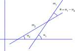
Figure 4.9: Two lines with inclinations a\ and a 2 < ct\ and slopes mi and m 2 . An angle of intersection is 9 = a.i — a 2 .
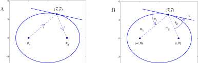
Refer to Figure 4.8B. Assume an equation of the ellipse is b 2 x 2 + a 2 y 2 = a 2 6 2 , a > b > 0. Then the focal points will be at (—c, 0) and (c, 0) where c = \/a 2 — b 2 . Let (x, y) denote a point of the ellipse. In order to establish the reflective property of ellipses, it is sufficient to show that the angle of incidence, Q\ is equal to the angle of reflection, 6 2 .
a. Find the slope, m, of the tangent at (x,y).
b. Show that
tan6*!
c. Write a similar expression for tan# 2 –
d. For the algebraically bold. Show that tan6^ = tan(9 2 –
e. Both tangents are positive, both angles are acute, and the angles are equal.
4.7 Summary of Chapter 4
We have defined continuity of a function, shown that if a function F has a derivative at a point x in its domain then F is continuous at x, and used this property to prove the Power Chain Rule,
PCR: [u n (t)]’= nu n 1 (t) x u'{t).
We proved PCR for all positive integers, n. In Exercises 4.3.3 and 4.3.4 you showed PCR to be true for all rational numbers, n. In fact, PCR is true for all numbers, n. We then used the power chain rule to solve some problems.
Exercises for Chapter 4, Continuity and the Power Chain Rule.
Chapter Exercise 4.7.1 Compute the derivative of P. a. P(t) = 3t 2 -2t + 7 b. P(t) = t+| d. P{t) = (t 2 + lf e. P(t) = ^/2~t + l
g. p(t) = ^ h Pit) = (l+vty 1
1/3
j. P(t) = (l + 30 1/d k. Pit)
l + Vi
Chapter Exercise 4.7.2 In “Natural History”, March, 1996, Neil de Grass Tyson discusses the discovery of an astronomical object called a “brown dwarf”.
“We have suspected all along that brown dwarfs were out there. One reason for our confidence is the fundamental theorem of mathematics that allows you to declare that if you were once 3’8″ tall and are now 5’8″ tall, then there was a moment when you were 4’8” tall (or any other height in between). An extension of this notion to the physical universe allows us to suggest that if round things come in low-mass versions (such as planets) and high-mass versions (such as stars) then there ought to be orbs at all masses in between provided a similar physical mechanism made both.
What fundamental theorem of mathematics is being referenced in the article about the astronomical objects called brown dwarfs? What implicit assumption is being made about the sizes of astronomical objects? (For future consideration: Is the number of ‘orbs’ countable?)
Chapter Exercise 4.7.3 In a square field with sides of length 1000 feet that are already fenced a farmer wants to fence two rectangular pens of equal area using 400 feet of new fence and the existing fence around the field. What dimensions of lots will maximize the area of the two pens?
Chapter Exercise 4.7.4 You must cross a river that is 50 meters wide and reach a point on the opposite bank that is 1 km up stream. You can travel 6 km per hour along the river bank and 1 km per hour in the river. Describe a path that will minimize the amount of time required for your trip. Neglect the flow of water in the river.
Chapter Exercise 4.7.5 Find the point of intersection of the tangents to the ellipse
x 2 /22A + y 2 /128 = 1/7 at the points (2,4) and (5, -2).
Chapter 5
Derivatives of Exponential and Logarithmic Functions
5.1 Derivatives of Exponential Functions.
Exponential functions are often used to describe the growth or decline of biological populations, distribution of enzymes over space, and other biological and chemical relations. The rate of change of exponential functions describes population growth rate, decay of chemical concentration with space, and rates of change of other biological and chemical processes.
The exponential function E(t) = 2* (where the base is 2 and the exponent is t) is quite different from the algebraic function, P(t) = t 2 (where the base is t and the exponent is 2). P(t) = t 2 is well defined for all numbers t in terms of multiplication, P(t) = t x t. However, in elementary courses 2* is defined only for t a rational number. For the irrational number \/2 = 1.4142135 ■ ■ ■, for example,
CHAPTER 5. EXPONENTIAL AND LOGARITHMIC FUNCTIONS
213
2^ is the number to which the sequence 2 L4 , 2 1,41 , 2 L414 , 2 L4142 , ■ ■ ■ approaches. We will not formalize this idea, but will assume that 2* is meaningful for all numbers t.
Shown in Table 5.1 are computations and a graph directed to finding the rate of growth of E(t) = 2* at t = 2. We wish to find a number m 2 so that
lim
b^2
2 b -2 2 b-2
m 2 .
Table 5.1: Table and Graph of E(t) = 2 t near t = 2.
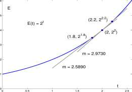
Explore 5.1.1 Compute the two entries corresponding to b = 1.99 and b = 2.01 that are omitted from Table 5.1. ■
Within the accuracy of Table 5.1, you may conclude that vri2 should be between 2.7724926 and 2.7726848. The average of 2.7724926 and 2.7726848 is a good estimate of m 2 .
^[2,1.9999] + ra[2,2.oooi] = 2.7724926 + 2.7726848 = 77258g7 2 2
We will find in Example ?? that correct to 11 digits, the rate of growth of E(t) at t = 2 is 2.7725887222. As approximations to E'(2), 2.7724926 and 2.7726848 are correct to only five digits, but their average, 2.7725887, is correct to all eight digits shown. Such improvement in accuracy by averaging left and right difference quotients (defined next) is common. For P a function, the fraction,
P{b) – P(a) b — a
is called a difference quotient for P. If h > 0 then the backward, and centered, and forward difference quotients at a are
Backward Centered Forward
P(a) – P(a – h) P(a + h) – P(a – h) P(a + h) – P(a)
h 2h h
CHAPTER 5. EXPONENTIAL AND LOGARITHMIC FUNCTIONS
214
Assuming the interval size h is the same in all three, the centered difference quotient is the average of the backward and forward difference quotients.
P(a -h)- P(a) + P(a + h) – P(a)
-h
h
-P(a-h) + P{a) P(a + h)-P(a) h h
-P(a -h) + P(a) + P(a + h) – P(a) 2h
P(a + h)- P{a – h) 2h
(5.1)
The graphs in Figure 5.1 suggest, and it is generally true, that the centered difference quotient is a better approximation to the slope of the tangent to P at (a, P(a)) than is either the forward or backward difference quotients. Formal analysis of the errors in the two approximations appears in Example 12.7.3, Equations 12.22 and 12.23. We will use the centered difference quotient to approximate E\a) throughout this chapter.
A
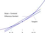
B
Slope = Centered Difference Quotient
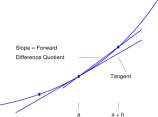
Slope = Forward Difference Quotient
Tangent
Figure 5.1: The centered difference quotient shown in A is closer to the slope of the tangent at (a, f(a)) than is the forward difference quotient shown in B.
Using the centered difference approximation, we approximate E'{t) for E(t) = 2* and five different value of t, —1, 0, 1, 2, and 3.
E'(-l) E'(0) E'(l) E'{2) E>(3)
Centered diff quot 2-1+0.0001 _ 2-1-0.0001
0.0002
E’it) =
0.34657359
0.69314718
1.3862944
2.7725887
5.5451774
E\t) E(t) 0.35 h
0.69 1.39 2.77 5.55
1
2 4
CHAPTER 5. EXPONENTIAL AND LOGARITHMIC FUNCTIONS
215
Explore 5.1.2 Do This. An elegant pattern emerges from the previous computations. To help you find it the last two columns contain truncated approximations to E'(t) and the values of E(t). Spend at least two minutes looking for the pattern (or less if you find it). ■
The pattern we hope you see is that
E'{t) = E'(0) E(t)
We will soon show that for E(t) = 2′, E'(t) = E'(0) E(t), exactly. Meanwhile we observe that E'(0) = 0.69314718 and
E'(0) E(-l) = 0.69314718 \ = 0.34657359 = E'(-l),
E'(0) E(l) = 0.69314718 x 2 = 1.38629436 = E'(l),
E'(0) E{2) = 0.69314718 x 4 = 2.77258872 = E'(2), and
E'(0) E(3) = 0.69314718 x 8 = 5.54517744 = E'(3), which supports the pattern.
Explore 5.1.3 Let E(t) = 3*. Use the centered difference quotient to approximate E'(t) for * = -1, 0, 1, 2, 3. Test your numbers to see whether E'(t) = E'(0) E(t). m
The previous work suggests a general rule:
Theorem 5.1.1 If E(t) = B l where B > 0, then
E\t) = E'(0) E(t).
(5.2)
Proof: For E(t) =B\B> 0,
E\t)
lim
B t+h _ B t h
lim
h->0
B t B h _ B t
= B l lim
h
B h – B°
lim
h->0
B f (B h – l)
h
h-,0 h
= E(t) E'(0)
End of proof.
The preceding argument follows the pattern of all computations of derivatives using Definition 3.23. We write the difference quotient, F ( t + h )F ( t ) ; balance h in the denominator with some term in the numerator, and let h — > 0. In Chapters 3 and 4 we always could factor an h from
CHAPTER 5. EXPONENTIAL AND LOGARITHMIC FUNCTIONS
216
the numerator that algebraically canceled the h in the denominator. In this case, there is no factor, h, in the numerator, but
as/wO, >E'(0),
and h in the denominator is neutralized (even though we do not yet know E'(0)).
Exercises for Section 5.1 Derivatives of Exponential Functions.
Exercise 5.1.1 (a) Compute the centered difference
P(a + h) – P(a-h) 2h ‘
which is an approximation to P'(a), for P(t) = t 2 and compare your answer with P'(a). (b) Compute the centered difference
P{a + h) – P(a – h) 2h
for P(t) = 5t 2 — 3t + 7 and compare your answer with P'(a).
Exercise 5.1.2 Technology Sketch the graphs of y = 2* and y = 4 + 2.7725887(t – 2)
a. Using a window of 0 < x < 2.5, 0 < y < 6.
b. Using a window of 1.5 < x < 2.5, 0 < y < 6.
c. Using a window of 1.8 < x < 2.2, 3.3 < y < 4.6. Mark the point (2,4) on each graph.
Exercise 5.1.3 Let E(t) = 10*.
a. Approximate E'(0) using the centered difference quotient on [—0.0001,0.0001].
b. Use your value for E'{0) and E'(t) = E'{0) E(t) to approximate E'{-1), E'{1), and E'(2).
c. Sketch the graphs of E(t) and E'(t).
d. Repeat a., b., and c. for E(t) = 8*.
Exercise 5.1.4 Let E(t) = (|)*.
a. Approximate E'(0) using the centered difference quotient on [—0.0001,0.0001].
b. Use your value for E'(0) and E'(t) = E'(0) E(t) to approximate E'{-1), E'(l), and E'{2).
c. Sketch the graphs of E(t) and E'(t).
CHAPTER 5. EXPONENTIAL AND LOGARITHMIC FUNCTIONS
217
Exercise 5.1.5 Find (approximately) equations of the lines tangent to the graphs of
a. y = 1.5* at the points (-1,2/3), (0,1), and (1,3/2)
b. y = 2* at the point (-1,1/2), (0,1), and (1,2)
c. y — 3* at the point (—1,1/3), (0,1), and (1,3)
d. y = 5* at the point (-1,1/5), (0,1), and (1,5)
Exercise 5.1.6 Suppose a bacterium Vibrio natriegens is growing in a beaker and cell concentration C at time t in minutes is given by
C(t) = 0.87 x 1.02* million cells per ml
a. Approximate C(t) and C'(t) for t — 0, 10, 20, 30, and 40 minutes.
b. Plot a graph of C'(t) vs C(t) using the five pairs of values you just computed.
Exercise 5.1.7 Suppose penicillin concentration in the serum of a patient t minutes after a bolus injection of 2 g is given by
P(t) = 200 x 0.96* /ig/ml
a. Approximate P(t) and P'(t) for t — 0, 5, 10, 15, and 20 minutes.
b. Plot a graph of P'(t) vs P{t) using the five pairs of values you just computed.
5.2 The number e.
The implication
For E(t) = B* =>• £?'(*) = E'(0) x
would be even simpler if we find a value for B so that E'(0) = 1. We next find such a value for B. It is universally denoted by e and
e is approximately 2.71828182845904523536; e is not a rational number.
Then for E(t) = e*, £'(0) = 1 so that E'(t) = E'(0) E(t) = 1 x E(t) = e{t).
Thus
a very important result.
Our goal is to find a base, e, so that
Because
t=o
0.69341 and
t=o
t=o
1.098612,
we think the base e that we seek is between 2 and 3 and perhaps closer to 3 than to 2.
CHAPTER 5. EXPONENTIAL AND LOGARITHMIC FUNCTIONS
218
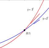
-0.5
0.5
Figure 5.2: Graphs of exponential functions, y = 2*, and y = 3* and segments of the tangents for each. The tangents have slopes approximately 0.69341 and 1.098612, respectively.
Explore 5.2.1
and
t=o
t=o
and the line of slope 1 through (0,1) is tangent to the graph of y = e l . Draw a line of slope 1 through the point (0,1). Then draw a graph of an exponential function whose tangent at (0,1) is the line you drew. Compare your graph with those in Figure 5.2. ■
Assuming that
it must be that
t=o
lim
/i-»0
h
lim
h->0
1.
Intuitively then, for h close to zero
1.
e h -l
h
e h -l
h.
(i + /0*
We will use this to explore e, and in Subsection 5.2.1 we will find that
e = lim(l + h) h .
(5.3)
Values of (1 + h)h for progressively smaller values of h are shown in Table 5.2. As h > 0 decreases toward 0, (1 + h) l l h increases. We show in Subsection 5.2.1 that (1 + h)h approaches a number as h approaches 0, and we denote that number by e.
Explore 5.2.2 Compute A = (1 + hfl h for h = 0.0001, h = 0.00001, and h = 0.000001. ■
Your last estimate of A should be approximately 2.71828047, which is an estimate correct to 6 digits of the irrational number e that we are seeking.
CHAPTER 5. EXPONENTIAL AND LOGARITHMIC FUNCTIONS
219
Table 5.2: Approximations to the number e. As h moves toward 0, A = (1 + h) l l h increases toward e.
Definition 5.2.1 The number e The number e is defined by
lim (1 + h ) s = e Correct to 21 digits, e = 2.71828 18284 59045 23536
We show in Subsection 5.2.1 that if h = \ for n an integer greater than 2
(1 + < e < (1
(5.4)
and we assume the inequalities are valid for all 0 < h < 1/2. Using these inequalities it is easy to show that the function E(t) = e* has the property that E'(0) = 1. We write, for 0 < h < 1/2,
As /i -> 0
Thus for E(t) = e\ E'(0) = I.
CHAPTER 5. EXPONENTIAL AND LOGARITHMIC FUNCTIONS
220
Because of Theorem 5.1.1, E'(t) = E'(0) x E(t) = e*, we have another Primary Formula for computing derivatives:
= e
Exponential Rule
(5.5)
Strategy for computing derivatives: Now we can use three Primary Formulas (Constant, Power, Exponential) and three Composition Formulas (Sum, Constant Factor, Power Chain) to compute derivatives. In finding derivatives of functions with many terms, students sometimes ask what derivative rule to use first and in subsequent steps. We think of the derivative procedure as peeling the layers off of an onion – outside layer first, etc. For example, to compute the derivative of F(t) = (2 + 3t 2 + 5e’) 3 we write:
F'(t)
2 + 3t 2 + 5e* ) 3
(5.6)
Symbolic Identity Power Chain Rule Sum Rule
Constant Rule
Constant Factor Rule
Power Rule
Exponential Rule
Think how the expression for F in the previous example, F(t) = (2 + 3t 2 + 5e*) 3 , is evaluated. Given a value for t you would compute t 2 and multiply it by 3 and you would compute e* and multiply it by 5, and then you would sum the three terms. The last step (outside layer) in the evaluation is to cube the sum. The first step in computing the derivative is to ‘undo’ that cube (use the Power Chain Rule).
The next step is to undo the sum with the Sum Rule. The next step is not uniquely determined; we worked from left to right and chose to evaluate [2]’.
In evaluating 3t 2 and 5e’, the last step would be to multiply by 3 or 5 – the first step in finding the derivative of 3t 2 and 5e* is to factor 3 and 5 from the derivative (Constant Factor Rule),
3t 2
3 t 2
5e*
5 e*
CHAPTER 5. EXPONENTIAL AND LOGARITHMIC FUNCTIONS
221
Usual course of events.
In computing derivatives, use the Composition Formulas first and the Primary Formulas last.
5.2.1 Proof that lim (1 + h) 1/h exists.
h^O v ‘
Our goal is to prove that
lim (1 + h)
We only consider the values of h for h
1/h exists, where n a positive integer, however, and show that
lim ( 1 H— I exists. nj
You may accept this information without proof and proceed to the section exercises. The material of this subsection is very important, however, and deserves your substantial independent effort.
Explore 5.2.3 Do this! Explain the MAT relevance to our goal, h
close all;clc;clear h= [0.01:0.01:1]; y=(l+h).~(l./h); plot(h,y,’k’,’linewidth’,2) holdOon’) For n = 1:8 z=(l+l/n)~n;
plot(l/n,z,’ks’,’linewidth’,2) end
axis([0 1.1 1.8 3])
AB program and the graph it creates and their
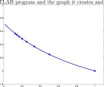
The graph in Explore 5.2.3 may convince you that lim (1 + h) 1 ^ exists and that there is
nothing left to prove. But it is the existence of a number that is the limit that is in question and that existence requires a crucial property of the number system called completeness.
CHAPTER 5. EXPONENTIAL AND LOGARITHMIC FUNCTIONS
222
Axiom 5.2.1 Completeness property of the number system. If Si and
S2 are two sets of numbers and
1. Every number belongs to either Si or S2, and
2. Every number of Si is less than every number of S 2 ,
then there is a number C such that C is either the largest number of Si or C is the least number of S 2 .
The statement of the Completeness Axiom by Richard Dedekind in 1872 greatly increased our understanding of the number system. In this text, the word ‘set’ means a nonempty set.
As noted above, we only consider values of h — 1/n where n is a positive integer and we define
( 1 V
s n — 1H— and prove that lim s n exists. V nj ‘
That a sequence of numbers si, s 2 , s 3 • • • is bounded means that an open interval (A, B) 1 contains every number in si, s 2 , S3 • • •; A is called a lower bound and B is called an upper bound of
si, s 2 , s 3
The sequence {1,4,9,16, 25, • • •} has no upper bound and is not bounded. The sequence {1, rj, \, ■ • •} is bounded by the numbers 0 and 2. The sequence {1, —2, 3, —4, 5, —6, • • •} has neither a lower bound nor an upper bound and is not bounded.
For this section we prove:
Theorem 5.2.1 If si < s 2 < s 3 < ■ ■ ■ is a bounded nondecreasing sequence of numbers there is a number s such that lim s n = s.
To prove Theorem 5.2.1 we need a clear definition of limit of a sequence.
Definition 5.2.2 A number s is the limit of a number sequence si, s 2 , S3 • • • means that if (u,v) is an open interval containing s there is a positive integer N such that if n is an integer greater than N, s n is in (u,v). It is sometimes said that si, s 2 , s 3 • • • converges to s or approaches s.
Example 5.2.1 The limit of the sequence {1, r>, ^, • • } is zero. If (u, v) contains 0, v is greater than zero and there is 2 a positive integer N that is greater than 1/v. Therefore, ifn>N,n>l/v so that 1/n < v, and u < 0 < 1/n < v, so ^ is in (u,v)). m
Proof of Theorem 5.2.1. Suppose si, s 2 , s 3 • • • is a nondecreasing sequence bounded by A and B. Let Si be the set of numbers x for which some number of Si, s 2 , s 3 • • • is greater than x. A is a member of Si and B is not a member of Si. Let S 2 denote all of the numbers not in Si Clearly every number is in either Si or S 2 .
1 If A and B are numbers with A < B, the open interval (A, B) consists of all the numbers between A and B; the closed interval [A, B] consists of A, B, and all of the numbers between A and B.
2 This is called the Archimedean property of the integers and may be treated as an axiom also. It is, however, a consequence of the Completeness Axiom, Exercise 5.2.11
CHAPTER 5. EXPONENTIAL AND LOGARITHMIC FUNCTIONS
223
To use the Completeness Axiom we must show that every number of Si is less than every number of S2. Suppose not; suppose there is a number x of Si that is greater than a number y of £2■ Then x has the property that some number, s n , say of si, s 2 , S3 • • • is greater than x and y is not in Si so no number of Si, s 2 , S3 • • • is greater than y. However, the supposition that y < x and x < s n , leads to y < s n which is a contradiction. Therefore every number of Si is less than every number of S2.
By the Completeness Axiom, either Si has a largest number or S2 has a least number. Suppose
51 has a largest number, L\. By definition of Si there is a member s n of Si, s 2 , s 3 • • • greater than L x . Now ^ l 2″ Sn is less than s n so ^ l j Sn is in L x . But ^ l j S ” is greater than Li so Li is not the largest member of Si, which is a contradiction; Si does not have a largest number. Therefore
52 must have a least number, L 2 .
We prove that Si, s 2 , S3 • • • approaches L 2 . Suppose (u,v) is an open interval containing L 2 . Then u is less than L 2 so belongs to Si and there is a number, Sn in Si, S2, S3 • • • that is greater than u. Because si, S2, S3 • • • is increasing, if n is greater than N, Sn < s n . No number of si, S2, S3 • • • is greater than L 2 . Therefore if n is greater than N,
u < sn < s n < L 2 < v
and the definition that si, S2, S3 • • • approaches L 2 is satisfied. End of proof.
Example 5.2.2 We can use Theorem 5.2.1 to show a useful result, that if a is a number and 0 < a < 1, then the sequence x n = a n converges to zero.
Proof. We assume the alternate version of Theorem 5.2.1 that If si > s 2 > s 3 > • • • is a bounded nonincreasing sequence of numbers there is a number s such that lim s n = s.
n— >oo
Because 0 < a < 1 and x n+ i < x n , and it follows that
nonincreasing (actually decreasing) sequence. Then {x n } approaches the greatest lower bound, s of {x n }.
If s < 0, then (2s, 0) is an open interval containing s and there is a number, x m in {x n } in (2s, 0). Then x m = a m is negative which is a contradiction.
Suppose s > 0. Because 0 < a < 1), the number s/a is greater than s and there is a number, x m in {x n } such that x m < s a . Because s is a lower bound on {x n }, s < x m . Then
s < x m < s/a, s < a rn < s/a, s ■ a < a m+1 < s, x m+ i < s.
But this contradicts the condition that s is a lower bound on {x n }.
We conclude that s, the greatest lower bound on {x n }, is zero and {x n } converges to 0. ■
Now to the number, e. We are to show that lim (1 + — ) n exists. We will show that
1. The sequence s n = (l + ^ is an increasing sequence.
2. The sequence t n — (l + , n > 1, is a decreasing sequence.
3. For every n > 1, s n < t n .
4. As n increases without bound, t n — s n approaches 0.
Conditions 1 and 3 show that Si < S2 < S3 < • • • is a bounded increasing sequence and therefore approaches a number s. That number s is the number we denote by e. Conditions 2 and 3 show that ti > t 2 > £3 > • • • is a bounded decreasing sequence and it follows from Theorem 5.2.1 3 that
3 Observe that —t\ < —t 2 < —t 3 < • • • is a bounded increasing sequence and there is a number —t such that —ti < —£2 < —£3 < • • • approaches —£.
CHAPTER 5. EXPONENTIAL AND LOGARITHMIC FUNCTIONS
224
there is a number t such that t\ > t 2 > t 3 > ■ ■ ■ converges to t By condition 4 above, t = s.
The proofs of conditions 3 and 4 above are left as exercises. Our argument for conditions 1 and 2 is that of N. S. Mendelsohn 4 based on the following theorem. The theorem is of general interest and we prove it in Subsection 8.1.2, independently of the work in this section.
Theorem 5.2.2 If a x , a 2 , ■ ■ ■, a n is a sequence ofn positive numbers then
a\ + a 2 + • • • a
– > v^i^ • • • a n (5.7)
Th
with equality only when a± — a 2 — • ■ ■ — a
n-
The left side of inequality 5.7 is the arithmetic mean and the right side is the geometric mean of ai, a 2 , • • •, a n . The theorem states that the arithmetic mean is greater than or equal to the geometric mean.
1. Proof that (l + ±)” is increasing. Consider the set of n + 1 numbers
1 1 1
1 + -, 1 + – ••• 1 + –
n n n
They are not all equal and they have an arithmetic mean of 1 + l/(n + 1) and a geometric mean of (1 x (l + l/n) n ) 1/(n+1) . Then
l + ^Xll + l/O 1 ^ or (l + ^y) >(l + l/n) B
Hence s n+ i > s n and the sequence s±, s 2 , • • • is increasing.
2. Proof that (l + ^^^j is decreasing. Consider the set of n + 1 numbers
n — 1 n — 1 n — 1
They have an arithmetic mean of n/(n + 1) and a geometric mean of (1 x ( (n — l)/n ) n ) and
n f n — 1 ^ “/(“+!)
>
71+1 V 71
By taking reciprocals this becomes
Ti + 1 / n W(n+i) / l \ ri+1
< 7 or 1 + < 1 +
n V n — 1 / \ (n +1) — 1 y V n — 1
It follows that t n+ i < t n and ti, t 2 , • ■ • is decreasing. End of proof.
We have shown that lim (1 H— ) n = e We claim the more general result that
lim (1 + h) l l h = e. We are encouraged to this claim by an identification of h — 1/n, but there are
other values of h to consider that are not reciprocals of integers. You will show in Exercise 12.2.5 that the slope of the graph in Explore 5.2.3 is negative and this provides a way to complete the proof that lim (1 + h) l ^ h = e. In the suggested solution to that exercise, [In u(x) ]’ is used.
log 10 u(x) could be used equally well, so that the argument is not dependent on the number e.
CHAPTER 5. EXPONENTIAL AND LOGARITHMIC FUNCTIONS
225
Explore 5.2.4 Explain the MATLAB program and the graph it creates and their relevance to the previous paragraph. H
close all;clc;clear h= [0.01:0.01:1];
N=[10, 11, 13,17,20,25,33,50,100];
0.6
F=0*h;
for i = 1:9
F(N(i))=l;
end
plot(h,F,’kd’,’linewidth’,2) axis([0 1.1 -0.1 1.1])
&0 00 0 0
Exercises for Section 5.2, The number e.
Exercise 5.2.1 Derivatives of functions are computed below. Identify the rule used in each step. In a few steps the rule is an algebraic rule of exponents and not a derivative rule.
a. [5t 4 -7e*]’ b. [5t 4 ]’- [7e*]’ 5[t 4 ]’-7[e t ]’ 5 x 4t 3 – 7 [e*]’ 5 x 4t 3 – 7 x e*
(l + e 4 ) 8 (l + e’^l + e*]’ (1 + e t ) 7 (\l]’ + \e t }’
(l + e*) 7 (0+[e*]’ (l + e*) 7 (0 + e*)
c. e
3< ■
ieUl + e t ) 7
t\3
e l )
3(ef [e«]’ 3(e*) 2 x e* 3e 2 * x e* 3e 3 *
Exercise 5.2.2 Differentiate (means compute the derivative of) P. Use one rule for each step and identify the rule as, C (Constant Rule), t n (t n Rule), S (Sum Rule), CF (Constant Factor Rule), PC (Power Chain Rule), or E (Exponential Rule). For example,
[vrr 2 – 5(e t ) 7 ]’
CHAPTER 5. EXPONENTIAL AND LOGARITHMIC FUNCTIONS
226
Careful, the next two are easier than you might first think.
i. p(t) = 5e 3 j. P(t) = 10 x 7T 2
Exercise 5.2.3 Draw the graphs of
yi(t) = e t y 2 it) = t 2 y 3 it) = t 3 y 4 (t) = t A -l<t<5
The graphs are close together near t — 0 and increase as t increases. Which one grows the most as t increases? Expand the domain and range to — 1 < t < 10, 0 < y < 25,000, and answer the same question.
Exercise 5.2.4 Draw the graphs of
t 2 t 3 t 4
y(t)=e t and p(t) = 1 + t + – + – + — Set the domain and range to — 1 < t < 2. and 0 < y < 8.
Exercise 5.2.5 We found a base e so that E(t) = e* has the property that the rate of change of E at 0 is 1. Suppose we had searched for a number B so that the average rate of change of E B (t) = B l on [0,0.01] is 1:
£ B (0.01) – E B (0) _ B 0 01 – B° _ B 0 01 – 1 _
m °001 ” om – o.oi – ~^oT~ -L
a. Solve the last equation for B.
b. Solve for B in each of the equations:
^0.001 _ i £>0.00001 _ -y ^o.ooooooi _ i
o.ooi ~ 1 o.ooooi ~ 1 o.ooooooi ~ 1
Exercise 5.2.6 On a popular television business news channel, an analyst exclaimed that “XXX stock has gone parabolic.” Is there some sense in which this exclamation is more exuberant than “XXX stock has gone exponential?”
CHAPTER 5. EXPONENTIAL AND LOGARITHMIC FUNCTIONS
227
Exercise 5.2.8 We introduced the power chain rule = n(u(x)) n ~ l [u(x)]’ for fractional
and negative exponents, n, in Section 4.3.1 (see Exercises 4.3.3 and 4.3.4). Use these rules when necessary in the following exercise. Compute y'(x) and y”{x) for
Exercise 5.2.9 Identify the errors in the following derivative computations. (t4 + r i) 7 l / b. [5t 7 + 7r 5 ]’ c. [10t 8 + 8e 5 *]’
7(t 4 + r 1 ) 6 [t 4 + r 1 ]’
a.
7(t 4 + r 1 ) 6 [t 4 ] , + [r 1 ] / 7(t 4 + r 1 ) 6 4t 3 + (-i)t
28t 3 (t A + t~ l f -t
5[t 7 ]’ + 7[r 5 ]’ 10[t 8 ]’ + 8[e 5 *]’
i + _^e 4t 3 + ( _ 1)r 2 5 x 7f + 7 x (-5)r 4 10 x 8t 7 + 8 x 5e 4 *
,. . ; f _ n6 + _ 2 35 (* 6 / ‘) 40(2t 7 + e 4t )
Exercise 5.2.10 Locate the point (0, e) on the graph in Explore 5.2.3
Exercise 5.2.11 Use the Completeness Axiom 5.2.1 to show that the positive integers do not have an upper bound. (This is called the Archimedean Axiom).
Exercise 5.2.12 Argue that if Si and S2 are two sets of numbers and every number is in either Si or S2 and every number in Si is less than every number in S2 then it is not true that there are numbers Li and L2 such that Li is the greatest number in Si and L2 is the least number in S2. Is this a contradiction to the Completeness Axiom?
Exercise 5.2.13 Let S2 denote the points of the X-axis that have positive x-coordinate and Si denote the points of the X-axis that do not belong to S2. Does S2 have a left most point?
Exercise 5.2.14 Suppose S 2 is the set of numbers to which x belongs if and only if x is positive and x 2 > 2 and Si consists of all of the other numbers.
CHAPTER 5. EXPONENTIAL AND LOGARITHMIC FUNCTIONS
228
2. Give an example of a number in Si.
3. Argue that every number in Si is less than every number in S2.
4. Which of the following two statements is true?
(a) There is a number C which is the largest number in S\.
(b) There is a number C which is the least number in £2.
5. Identify the number C in the correct statement of the previous part.
Exercise 5.2.15 Suppose your number system is that of Early Greek mathematicians and includes only rational numbers. Does it satisfy the Axiom of Completion?
Exercise 5.2.16 Show that if n > 2 and s n = (l + ^ and t n — (l + then
a. For every n s n < t n .
b. Justify the steps (i) to (iv) in
<<n °n
(1 + 5^)”-(! + *)”
. n-1
= <
= <
1
n(n — 1)
x n x 1 +
n-l
1
n — 1
x 4
c. As n increases without bound, t n — s n approaches zero.
5.3 The natural logarithm
(0
(ii)
(Hi) (iv)
The natural logarithm function, In, is defined for u > 0 by
A = ln-u = log e u <^=^> u = e x
(5.8)
The natural logarithm is the logarithm to the base e and the properties of logarithms for all bases apply:
CHAPTER 5. EXPONENTIAL AND LOGARITHMIC FUNCTIONS
229
The natural logarithm is keyed on most calculators as In or LN. Equation 5.12 shows that all logarithms may be calculated using just the natural logarithm. However, log 10 is also keyed on most calculators and the key may be labeled Log or LOG. But in MATLAB log(x) means natural logarithm of x.
Using Equation 5.13 we can express all exponential functions in terms of the base e. To see this, suppose B > 0 and E(t) = B l . Equation 5.13 states that
thiB
so we may write E(t) = B* as
E(t) = B l = (e lnB )’ = e For example, In 2 = 0.631472. For E(t) = 2 t we have
J E(t) = 2*=( e ln2 ) t = e tln2 = e 0
631472*
As a consequence, functions of the form E(t) = e kt , k a constant, are very important and we compute their derivative in the next section.
Example 5.3.1 We found in Chapter 1 that cell density (measured by light absorbance, Abs) of Vibrio natriegens growing in a flask at pH 6.25, data in Table 1.1, was described by (Equation 1.5)
Abs = 0.0174 x 1.032 Time
Using natural logarithm, we write this in terms of e as
Abs = 0.0174 x 1.032 Time
,ln 1.032
Time
Abs = 0.0174
Abs = 0.0174 [ e 0.03150]Timc Abs = 0.0174 e °-03150xTime
Equation 5.13
In 1.022 = 0.02176 Equation 5.11. ■
CHAPTER 5. EXPONENTIAL AND LOGARITHMIC FUNCTIONS
230
Exercises for Section 5.3, The natural logarithm.
Exercise 5.3.1 You should have found in Explore 1.6.1 that plasma penicillin during 20 minutes following injection of two grams of penicillin could be computed as
P(T) = 200 x 0.77 T T = index of five minute intervals.
a. Write P in the form of P(T) = 200 e~ kl T .
b. Write P in the form of P(t) = 200 e~ k ‘ 21 where t measures time in minutes.
Exercise 5.3.2 Use Equation 5.12, log d A = In A/ In d to compute log 2 A for A = 1, 2, 3, • • •, 10.
Exercise 5.3.3 We found in Section 1.3 that light intensity, Id, as a function of depth, d was given by
I d = 0.4 x 0.82 d
Find k so that I d = 0Ae kxd .
Exercise 5.3.4 Write each of the following functions in the form /(f) = A e
kt
a. f(t) = 5-10*
b. /(f) = 5-10-
c. /(f) = 7-2*
d. /(f) = 5-2-* e. fit) = 5 (I)* f. fit) = 5 (§)
-t
Exercise 5.3.5 Use the Properties of Logarithms, Equations 5.9 – 5.14 to write each of the following functions in the form /(f) = A + Bint.
a. /(f) = 5 log 10 f b. /(f) = 5 log 2 f 3
/(*)
7 log 5 5f
d. /(f) = 5 1og 10 3f e. /(f) = 3 1og 4 (f/2 3 ) f. /(f) = 3^(16^0)
5.4 The derivative of
Jz t
We have found the derivative of e*. Often, however, the function of interest is of the form C e where C and k are constants. In Example 5.3.1 of bacterial growth,
Abs = 0.0174 e^eTime
the constant C = 0.0174 and the function kt = 0.02176 Time. We develop a formula for
k t
,fc t
,fc t
e l )
k ( e*) fe_1 [ e*
k (e*) k e kt
(0
(«)
(in)
(5.15)
Because Equation 5.15
,fet
k e , is used so often, we call it another Primary Formula even
though we developed it without direct reference to the Definition of Derivative. Should you be limited to a single derivative rule, in the life sciences choose the e k 1 Rule exponential functions are ubiquitous in biology.
CHAPTER 5. EXPONENTIAL AND LOGARITHMIC FUNCTIONS
231
Explore 5.4.1 Were we to derive
,fc t
,fc t
The assertion in step (Hi) that
= k e kt from the Definition of Derivative, we would write:
= lim
e kb_ e ka
b^a b — a
e k b _ g fc a
= lim — — k
b^a k b — k a
= e ka k
lim
e kb_ e ka
= e
k a
b^a k b — k a
is correct, puzzles some students, and is worth your thought.
(0
(ii)
(Hi)
(5.17)
We can now differentiate functions like P(t) = 5t 7 + 3e 2t .
P'(t) = [5t 7 + 3e 2t ]’ A symbolic identity.
= [5t 7 ]’ +[3e 2 ‘]’ Sum Rule
= 5 [t 7 ]’ + 3 [e 2t ]’ Constant Factor Rule
= 5 x 7t 6 + 3 [e 2t ]’ Power Rule
= 35t 6 + 3e 2t 2 e kt Rule
= 35t 6 + 6e 2t
Example 5.4.1 We can also compute E'(t) for E(t) = I 1 .
[2*]’ = [(e ln2 )
e (ln2) t
e (ln2)t ln2 = 2 t ln2
We have an exact solution for the first problem of this Chapter, which was to find E'(2) for E(t) = 2*. The answer is 2 2 In 2 = 4 In 2. Also, E'(0) = 2° In 2 = In 2 which answers another question from early in the chapter, h
CHAPTER 5. EXPONENTIAL AND LOGARITHMIC FUNCTIONS
232
More generally, for b > 0,
[6*]’ = [(e lnb )
3 (ln6) t
= e^* In b = b l In 6
(it)
(Hi)
(iv)
(5.18)
We summarize this information:
t _ ut
b In b for b > 0.
(5.19)
Explore 5.4.2 This is very important. Show that if C and k are constants and P(t) = Ce kt then P'(t) = kP(t). m
Exercises for Section 5.4, The derivative of e kt .
Exercise 5.4.1 Give reasons for the steps (i) — (Hi) in Equation 5.15 showing that e kt k.
Exercise 5.4.2 Give reasons for the steps (i) — (iv) in Equation 5.18 showing that [&*]’ = b l In b.
Exercise 5.4.3 The function b l for b = 1 is a special exponential function. Confirm that the derivative equation [6*]’ = b l In b is valid for b = 1. Draw some graphs of b l for b = 1 and its derivative.
Exercise 5.4.4 Use one rule for each step and identify the rule to differentiate
a. P(t) = 3e 5 ‘ + 7r b. P(t) = y + ^
c. P(t) = 5* d. P(t) = e 2t e 3t
Simplify Part d before differentiating.
CHAPTER 5. EXPONENTIAL AND LOGARITHMIC FUNCTIONS
233
Exercise 5.4.5 Compute y'{x) or assert that you do not yet have forumlas to compute
y'(x) for
a. y(x) = e 5x b. y(x) = e~ 3x
c. y(x) = d. y(x) = (e x ) 2
e. y(x) = (e^) 2 f. y(x) = (e’ x ) 2
x —x
g.y(x) = e ~^~ h.y(x) =
i. y(x) = ^ e -o-06x + 3e -o.ix j y ^ = e (x 2 )
k. y(x) = v 7 ^ 1. y(x) = 8e-° moix -16e-° mix
m. y(x) = e 5 n. y(x) = \fe
o. y[x) = 10 x p. y(x) = 10~ x
q. y{x) = x 2 + 2 x r. y{x) = (e 5x + e~ 3x f
Exercise 5.4.6 Interpret e* 2 as e^ 2 \ Argue that
e (f,2) – e (a2) lim — k k — = e [a >
b^a b 2 – a 2
What is the ambiguity in the notation e” 2 . (Consider 4 32 .) Use parenthesis, they are cheap. However, common practice is to interpret e* as ).
Exercise 5.4.7 Argue that
lim V = ^
Exercise 5.4.8 Review the method in Explore 5.4.1 and the results in Exercises 5.4.6 and 5.4.7. Use Definition 3.22,
F(ci)
F'(a) = lim —^ —, to compute E'(a) for
b – a
a. E(t) = e 2t b. E{t) = e 2 ^ c. E(t) = e~*
I f ^ —i / i \ _ + 2
d. E{t) = e 2 e. E{t) = e« f. E{t) = e
Exercise 5.4.9 Consider the kinetics of penicillin that is taken as a pill in the stomach. The diagram in Figure Ex. 5.4.9(a) may help visualize the kinetics. We will find in Chapter 17 that a model of plasma concentration of antibiotic t hours after ingestion of an antibiotic pill yields an equation similar to
C(t) = he’ 2 * – 5e~ 3 * /xg/ml (5.20)
A graph of C is shown in Figure Ex. 5.4.9. At what time will the concentration reach a maximum level, and what is the maximum concentration achieved?
CHAPTER 5. EXPONENTIAL AND LOGARITHMIC FUNCTIONS
234
As we saw in Section 3.5.2 and may be apparent from the graph in Figure Ex. 5.4.9, the highest concentration is associated with the point of the graph of C at which C = 0; the tangent at the high point is horizontal. The question, then, is at what time t is C'(t) = 0 and what is C(t) at that time?
Figure for Exercise 5.4.9 (a) Diagram of compartments for oral ingestion of penicillin, (b) Graph of C(t) = 5e~ 2t — 5e~ 3 ‘ representative of plasma penicillin concentration t minutes after
ingestion of the pill.
Stomach
(a)
Exercise 5.4.10 Plasma penicillin concentration is
P(t) = 5 e” 0 3 ‘ – 5 e~ 0At
t hours after ingestion of a penicillin pill into the stomach. A small amount of the drug diffuses into tissue and the tissue concentration, C(t), is
C(t) = -e-°3t + 0.5e-° At + O.Se” 02 * /ig/ml
a. Use your technology (calculator or computer) to find the time at which the concentration of the drug in tissue is maximum and the value of C at that time.
b. Compute C'(t) and solve for t in C'(t) = 0. This is really bad, for you must solve for t in
0.3ea3 ‘-0.2ea4t -0.1e-°2 * = 0
Try this:
Let Z = e~ 0At then solve 0.3Z 3 – 0.2Z 4 – OAZ 2 = 0.
a Solve for the possible values of Z. Remember that Z = e~ 0At and solve for t if possible using the possible values of Z.
d. Which value of t solves our problem?
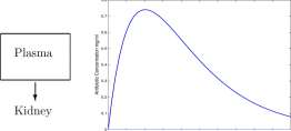
0 0.2 0.4 0.6 0.8 1 1.2 1.4 1.6 1.8 2
Time hours
(b)
CHAPTER 5. EXPONENTIAL AND LOGARITHMIC FUNCTIONS
5.5 The derivative equation P'(t) = k P(t)
A crucial property of exponential functions established by the e kt Rule is
235
Property 5.5.1 Proportional Growth or Decay. If P is a function defined by
P(t) = Ce kt where C and k are numbers, then
P'{t) = k P{t)
Proof that P(t) = Ce kt implies that P'(t) = kP(t):
P'(t)
Ce
kt
c
Ce kt k = kCe
kt
kP(t)
The reverse implication is also true, and is shown to be true in Chapter 17:
Property 5.5.2 Exponential Growth or Decay If P is a function and there is a number k for which
P'[t) = k P(t) for alH > 0
then there is a number C for which
P(t) = Ce kt
Furthermore,
C = P(0) so that P(t) = P(0) e
kt
In the preceding equations, k can be either positive or negative. When k is negative, it is more common to emphasize this and write —k and write P(t) = e~ kt , where in this context it is understood that A; is a positive number.
In Chapter 1, we examined models of population growth, light decay, and penicillin clearance, all of which were of the form
Pt+i — Pt — R Pt
and found that
Pt = Po R*
These are discrete time models in which the average rate of change of P t is proportional to P t . The exponential Growth or Decay Property 5.5.2 is simply a continuous time model in which the rate
CHAPTER 5. EXPONENTIAL AND LOGARITHMIC FUNCTIONS
236
of change of P(t) is proportional to P(t), and would be preferred in many instances. Bacterial populations may be visualized as growing continuously (and not in twenty minute bursts), the kidneys clear penicillin continuously (and not in five minute increments), and light decays continuously with depth (and not in one meter increments). Discrete time models are easy to comprehend and with short data intervals give good replications of data, but now that we know the definition of rate of change we can use continuous time or space models. The equation
dP
P’ = kP or P'(t) = kP(t) or — = kP
derives from many models of biological and physical processes including population growth, drug clearance, chemical reaction, decay of radio activity – any system which can be described by:
Mathematical Model 5.5.1 Proportional change. The rate of change of a quantity is proportional to the amount of the quantity.
For example in population studies, we commonly assume that
Mathematical Model 5.5.2 Simple population growth. The growth rate of a population is proportional to the size of the population.
Let P(t) be the size of a population at time, t. The component parts of the sentence in the Mathematical Model of simple population growth are symbolized by
a: The growth rate of a population : P'(t) b: is proportional to : = kx
c: the size of the population : P(t)
The sentence of the Mathematical Model is then written
P'(t) ^kx P(t)
a b c
From the property of Exponential Growth and Decay
P(t) = Cxe kt and if P(0) = P 0 is known P(t) = P 0 e kt (5.21)
In the event that the rate of decrease of a quantity, P(t), is proportional to the size of P(t), then because —P'(t) is the rate of decrease of P(t),
-P’ = k P{t), P’ = -k P{t), and P(t) = P 0 e~ kt ,
where A; is a positive number.
Example 5.5.1 A distinction between discrete and continuous models. Suppose in year 2000 a population is at 5 million people and the population growth rate (excess of births over deaths) is 6 percent per year. One interpretation of this is to let Pit) be the population size in millions of people at time t measured in years after 2000 and to write
Then, from the property of Exponential Growth or Decay 5.5.2, we may write
P(t)=P(0) e °06 * = 5e 0 06 *
P(t) = 5e 0 06 ‘ does not exactly match the hypothesis that ‘population growth rate is 6 percent per year’, however. By this equation, after one year,
P(l) = 5e°06xl = 5 e 0 06 = 5 x 1.06 1 8
The consequence is that during the first year (and every year) there would be a 6.18 percent increase, a contradiction.
The discrepancy lies with the model equation P'{t) = 0.6P(t). Instead, we may write
P(0) = 5 P\t) = k P{t)
where k is to be determined. Then from Exponential Growth or Decay 5.5.2 we may write
P(t) = 5 e kt
Now impose that -P(l) = 5 x 1.06, a 6 percent increase during the first year, and write
P(l) = 5 e kl = 5 x 1.06
This leads to
e kxl = 1.06
We take the natural logarithm of both numbers and get
ln(e fc ) = In 1.06 k = In 1.06 = 0.05827
Then
P(t) = 5 e 0 05827 ‘
gives a description of the population t years after 2000. Each annual population is 6 percent greater than that of the preceding year. The continuous model of growth is actually
P(0) = 5 P'{t) = (In 1.06) P(t) P'(t) = 0.05827P(t)
Explore 5.5.1 Show that for the discrete equations
P+i -P t = r P, with solution P t = P 0 (1 + r)\ the solution to the continuous equation
p'(f) = (]n(l + r))p(t), p(0) = Po agrees with p t at the integers. That is,
p(t)=P t , for i = 0,l,2,….
CHAPTER 5. EXPONENTIAL AND LOGARITHMIC FUNCTIONS
238
Explore 5.5.2 Bacterial density for v. natriegens grown in a nutrient solution at pH of 6.75 was given in Section 1.1 and are reproduced below. It was found that B t = 0.022 (5/3)* (Equation 1.4) matches the data very well. Find a number, k, such that the solution to B(0) = 0.022, B'{t) = kB{t) matches the solution at integer values of t.
The variable t is used ambiguously here. In B t , t is an index for 16-minute intervals and is 0, 1, 2, • • •, an integer. In B(t), t is a number greater than or equal to zero, but is also measuring time in 16-minute intervals. For example, B(2) is to be the bacterial density at the end of the second 16-minute interval, the same as B 2 . -8(1.5) is an estimate of the bacterial density at time 12 minutes, but Bi, 5 is not defined.
Time (min) Time index, t
The growth of a bank savings account is similar to this simplified model of population growth. If you deposited $5000 in 2000 at a true 6 percent annual interest rate, it may amount to
Pit) = 5000e a05827t
dollars t years after 2000. On the other hand, some banks advertise and compute interest on the basis of 6% interest with ‘instantaneous’ compounding, meaning that their model is
P'(t) = 0.06 P(t)
leading to
P(t) = 5000e a06t
They will say that their ‘APR’ (annual percentage rate) is 100 e a06 = 6.18 percent.
The solution to the discrete system
P 0 known P n+1 = K P n The solution of the continuous system p(0)=P o , p\t) = (\nK)p(t) For t — n, an integer, p(n) = P n .
is
Pn = P 0 K n .
IS
Pt
P 0 e ^ = P 0 K\
Example 5.5.2 Geologists in the early nineteenth century worked out the sequential order of geological layers well before they knew the absolute dates of the layers. Their most extreme
CHAPTER 5. EXPONENTIAL AND LOGARITHMIC FUNCTIONS
239
estimates of the age of the earth was in the order of 400 million years 5 , about 1/10 of today’s estimate of 4.54 ± 0.05 billion years 6 based on decay of radioactive material. Early applications of radiometric dating used the decomposition of uranium-238 first to thorium-234 and subsequently to lead-206. More recently potassium-40 decomposition has been found to be useful (and zircon decay is currently the best available).
Potassium-40 decomposes to both argon-40 and calcium-40 according to
9 ( 40 K) —> 40 Ar + 8 ( 40 Ca)
When deposited, volcanic rock contains significant amounts of 40 K but is essentially free of 40 Ar because 40 Ar is a gas that escapes the rock under volcanic conditions. Once cooled, some volcanic rock will become essentially sealed capsules that contain 40 K and retain the 40 Ar that derives from decomposition of the 40 K.
Mathematical Model 5.5.3 Potassium-40 decomposition. The rate of disintegration of 40 K is proportional to the amount of 40 K present.
If we let K(t) be the amount of 40 K present t years after deposition of rock of volcanic origin and Kq the initial amount of 40 K present, then
K(0) = K 0 , K'(t) = -rK(t)
where r is a positive constant. The minus sign reflects the disintegration of 40 K. From the equation we may write
K(t) = K 0 ert
The half-life of 40 K is 1.28 x 10 9 years, meaning that 1.28 x 10 9 years after deposition of the volcanic rock, the amount of 40 K in the rock will be \Kq. We use this information to evaluate r.
1 IS — IS a -r 1280000000 -A 0 — A 0 e
1
2
-r 1280000000
In 1 = -r 1280000000
2
r =
In 2
1280000000
K(t) = K 0 e
In 2 t 1280000000
Problem. Suppose a rock sample is found to have 5 x 10 14 40 K atoms and 2 x 10 13 40 Ar atoms. What is the age of the rock?
Solution. It is necessary to assume 7 that all of the 40 Ar derives from the 40 K, and that there has been no leakage of 40 K or 40 Ar into or out of the rock. Assuming so, then the number of 40 K atoms
5 Charles Darwin wrote in the Origin of Species that Earth was several hundred million years old, but he was opposed in 1863 by a dominant physical scientist, William Thompson (later to become Lord Kelvin) who estimated that Earth was between 24 and 400 million years old. His estimate was based on his calculation of the time it would take for Earth to cool from molten rock to today’s temperatures in the upper layers of the Earth. See article by Philip England, Peter Molnar, and Frank Richtcr, GSA Today, 17, 1 (January 1, 2007).
6 Wikipedia
CHAPTER 5. EXPONENTIAL AND LOGARITHMIC FUNCTIONS
240
that have decomposed (to either 40 Ca or 40 Ar) must be nine times the number of 40 Ar atoms, or 9 (2 x 10 13 ) = 1.8 x 10 14 atoms. Therefore
K 0 = 5 x 10 14 + 1.8 x 10 14 = 6.8 x 10 14
and
K(t) = 6.8 X 10 14 e~ “80000000 *
We want the value of t for which K(t) = 5 x 10 14 . Therefore,
5 x 10 14 = 6.8 x 10 14 e” 1280000000*
5
6\8
In 2
= e 1280000000
/
In 5 ln2 t
n 6T8 ~ ~ 1280000000 1
t = 568,000,000
The rock is about 568 million years old. h
5.5.1 Two primitive modeling concepts.
Primitive Concept 1. Suppose you have a barrel (which could just as well be a blood cell, stomach, liver, or lake or ocean or auditorium) and A(t) liters is the amount of water (glucose, plasma, people) in the barrel at time t minutes. If water is running into the barrel at a rate R\ liters/minute and leaking out of the barrel at a rate R2 liters/minute then
Rate of change of water = Rate water enters — Rate water leaves in the barrel the barrel the barrel
A'(t) = R 1 – R 2
L L L
min min min
Primitive Concept 2. Similar to Primitive Concept 1 except that there is salt in the water. Suppose S(t) is the amount in grams of salt in the barrel and C\ is the concentration in grams/liter of salt in the stream entering the barrel and C 2 is the concentration of salt in grams/liter in the stream leaving the barrel. Then
Rate of change of salt = Rate salt enters — Rate salt leaves in the barrel the barrel the barrel
S'(t) — C\ R\ — C2 R2
g g _L_ g L
min L min L min
Observe that the units are g/m on both sides of the equation. Maintaining a balance in units often helps to find the correct equation.
CHAPTER 5. EXPONENTIAL AND LOGARITHMIC FUNCTIONS
241
Example 5.5.3 Suppose a runner is exhaling at the rate of 2 liters per second. Then the amount of air in her lungs is decreasing at the rate of two liters per second. If, furthermore, the CO2 partial pressure in the exhaled air is 50 mm Hg (approx 0.114 g C0 2 /liter of air at body temperature of 310 K) 8 , then she is exhaling C0 2 at the rate of 0.114 g/liter x2 liters/sec = 0.228 g/sec. h
Example 5.5.4 Classical Washout Curve. A barrel contains 100 liters of water and 300 grams of salt. You start a stream of pure water flowing into the barrel at 5 liters per minute, and a compensating stream of salt water flows from the barrel at 5 liters per minute. The solution in the barrel is ‘well stirred’ so that the salt concentration is uniform throughout the barrel at all times. Let S(t) be the amount of salt (grams) in the barrel t minutes after you start the flow of pure water into the barrel.
Explore 5.5.3 Draw a graph of what you think will be the graph of S(t). In doing so consider
• What is 5(0)?
• Does S(t) increase or decrease?
• Will there be a time, £*, for which S(t*) = 0? If so, what is i*?
Solution. First let us analyze S. We use Primitive Concept 2. The concentration of salt in the water flowing into the barrel is 0. The concentration of salt in the water flowing out of the barrel is the same as the concentration C(t) of salt in the barrel which is
C( f ) = ^g/L
I ) 1Q0 6/
Therefore
Rate of change of salt in the barrel
Rate salt enters the barrel
Rate salt leaves the barrel
S'(t) S'(t)
Furthermore, S(0) = 300. Thus
C\ Ri 0x5
S(0) = 300
S'(t) = -0.05S(t).
C2 R2
100 L min
X 5;
L
From the Exponential Growth and Decay property 5.5.2,
S(t) = 300e-°05 ‘
Explore 5.5.4 . Draw the graph of S(t) = 300e~°’ 05 ‘ and compare it with the graph you drew in Explore 5.5.3. H ■
J^A x lliter x 44mol wt
m = 0.114g
0.08206 gas const x 310K
CHAPTER 5. EXPONENTIAL AND LOGARITHMIC FUNCTIONS
242
Example 5.5.5 Classical Saturation Curve.
Problem. Suppose a 100 liter barrel is full of pure water and at time t — 0 minutes a stream of water flowing at 5 liters per minute and carrying 3 g/liter of salt starts flowing into the barrel. Assume the salt is well mixed in the barrel and water overflows at the rate of 5 liters per minute. Let S(t) be the amount of salt in the barrel at time t minutes after the salt water starts flowing in.
Explore 5.5.5 Draw a graph of what you think will be the graph of S(t). In doing so consider
• What is 5(0)?
• Does S(t) increase or decrease?
• Is there an upper bound on S(t), the amount of salt in the barrel that will be in the barrel?
Solution: We analyze S; again we use Primitive Concept 2. The concentration of salt in the inflow is 3 g/liter. The concentration C(t) of salt in the tank at time t minutes is
at) = m
1; 100
The salt concentration in the outflow will also be C(t). Therefore
Rate of change of salt = Rate salt enters — Rate salt leaves in the barrel the barrel the barrel
S'(t) = C\ R\ — C2 R2
S'(t) = 3×5 – f^5
g g _L_ g L
min L min L min
Initially the barrel is full of pure water, so
(5.22)
5(0) = 0
We now have
5(0) = 0
S'(t) = 15-0.05 5(4)
This equation is not in the form of P'(t) = kP(t) because of the 15. Proceed as follows. Equilibrium. Ask, ‘At what value, E, of S(t) would S'(t) = 0?’ That would require
0 = 15- 0.05 E = 0, or E = 300 g.
E = 300 g is the equilibrium level of salt in the barrel. We focus attention on the difference, D(t), between the equilibrium level and the current level of salt. Thus
D(t) = 300 – S(t) and S(t) = 300 – D(t)
Now,
D(0) = 300 – 5(0) = 300 – 0 = 300
CHAPTER 5. EXPONENTIAL AND LOGARITHMIC FUNCTIONS
243
Furthermore,
S'(t) = [300 -D(t)}’ = -D'{t) We substitute into Equations 5.22
5(0) = 0 D(0) = 300
S'(t) = 15- 0.05 S(t) ~D'(t) = 15 – 0.05 (300 – D(t))
The equations for D become
D(0) = 300
D'(t) = -0.05 D(t)
This is in the form of the Exponential Growth and Decay Property 5.5.2, and we write
D(t) = 300e-° 05i
Returning to S{t) = 300 — D(t) we write
S(t) = 300 – D(t) = 300 – 300 e” 0 ‘ 05 *
The graph of S(t) = 300 — 300e~ 005t is shown in Figure 5.3. Curiously, the graph of S(t) is also called an exponential decay curve. S(t) is not decaying at all; S(t) is increasing. What is decaying exponentially is D(t), the remaining salt capacity, h
Explore 5.5.6 Show that if S{t) = 300 – 300 e -° 05i , then
5(0) =0, and S'(t) = 15 – 0.05 S(t).
350
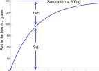
0 10 20 30 40 50 60 70 80 90
Time – minutes
Figure 5.3: The graph of S(t) = 300 — 300 e 005 * depicting the amount of salt in a barrel initially filled with 100 liters of pure water and receiving a flow of 5 L/m carrying 3 g/L. D(t) = 300 — S(t).
CHAPTER 5. EXPONENTIAL AND LOGARITHMIC FUNCTIONS
244
5.5.2 Continuous-space analysis of light depletion.
As observed in Chapter 1, light intensity decreases as one descends from the surface of a lake or ocean. There we divided the water into discrete layers and it was assumed that each layer absorbs a fixed fraction, F, of the light that enters it from above. This hypothesis led to the difference equation
Id+l — Id — —F Id
Light is actually absorbed continuously as it passes down through a (homogeneous) water medium, not in discrete layers. We examine the light intensity, I(x), at a distance, x meters, below the surface of a lake or ocean, assuming that the light intensity penetrating the surface is a known quantity, I 0 .
We start by testing an hypothesis about light transmission in water that appears different from the hypothesis we arrived at in Chapter 1:
Mathematical Model 5.5.4 Light Absorbance: The amount of light absorbed by a (horizontal) layer of water is proportional to the thickness of the layer and to the amount of light entering the layer (see Figure 5.4).
Water Surface
x + A x Ax
V
A£.
A x = Thickness
\|/'(x)
l(x+A x)
I
0 0.2 0.4 0.6 0.8 1 1.2
Figure 5.4: Diagram of light depletion below the surface of a lake or ocean. I(x) is light intensity at depth x due to light of intensity 7q just below the surface of the water.
The mathematical model of light absorbance implies, for example, that
1. The light absorbed by a water layer of thickness 2A is twice the light absorbed by a water layer of thickness A and
2. A layer that absorbs 10% of a bright light will absorb 10% of a dim light.
We know from experimental evidence that implication (1) is approximately true for thin layers and for low levels of turbidity. Implication (2) is valid for a wide range of light intensities.
Double Proportionality. From the mathematical model of light absorbance the light absorbed by a layer is proportional to two things, the thickness of the layer and the intensity of the light entering the layer. We handle this double proportionality by assuming that the amount of light
CHAPTER 5. EXPONENTIAL AND LOGARITHMIC FUNCTIONS
245
absorbed in a layer is proportional to the product of the thickness of the layer and the intensity of the light incident to the layer. That is, there is a number, K, such that if I(x) is the light intensity at depth x and I(x + Ax) is the light intensity at depth x + Ax, then
I(x + Ax) – I(x) = -K Ax x I(x) (5.23)
The product, K Ax x /(x), has the advantage that
1. For fixed incident light intensity, I{x), the light absorbed, I(x + Ax) — I(x), is proportional to the thickness, Ax, (proportionality constant = —K I(x)) and
2. For fixed thickness Ax, the light absorbed is proportional to the incident light, I(x) (proportionality constant = — K Ax).
Equation 5.23 can be rearranged to
7 <* ± A ;> – m =
Ax
The approximation (=) improves as the layer thickness, Ax, approaches zero.
. I(x + Ax) – I(x) ,
As Ax -> 0 — 1 — -> I (x)
Ax
and we conclude that
I'(x) = -KI(x) (5.24) The Exponential Growth and Decay Property 5.5.2 implies that
because I'(x) = —KI(x), I(x) = I Q e~ Kx (5.25)
Example 5.5.6 Assume that 1000 w/m 2 of light is striking the surface of a lake and that 40% of that light is reflected back into the atmosphere. We first solve the initial value problem
1(0) = 600 I'(x) = -KI(x)
to get
I(x) = 600 e~ Kx
If we have additional information that, say, the light intensity at a depth of 10 meters is 400 W/m 2 we can find the value of K. It must be that
J(10) = 600e^ xl ° = 400
The only unknown in the last equation is K, and we solve
600e^ xl ° = 400
£ -wk = 400/600 = 5/6
ln(V 10 ^) = In (2/3) — 10 K = In (2/3) K = 0.040557
CHAPTER 5. EXPONENTIAL AND LOGARITHMIC FUNCTIONS
246
Thus we would say that
I(x) = 600 e 0M0557x
If we know, for example, that 30 W/m 2 of light are required for a certain species of coral to grow, we can ask for the maximum depth, x, at which we might find that species. We would solve
I(x) = 30
60Q e -0.040557 x = 30
In (ea040557 s ) = In (30/600) -0.040557 x = In (1/20)
x = 73.9 meters
5.5.3 Doubling time and half-life
Suppose k and C are positive numbers. The doubling time of F(t) = Ce kt is a number t^bi such that
for any time t F(t + t dU ) = 2 x F(t). That there is such a number follows from
F(t + t M ) = 2xF(t) Ce k{t+t dbl ) = 2Ce kt
Ce kt e kt dbl = 2Ce
gfc tdM — 2
kt
t M = (5.26)
The half-life of F(t) = C e kt is a number thaif, usually written as ii/ 2 , such that
for any time t F(t + t 1/2 ) = 1 F(t). Using steps similar to those for the doubling time you can find that
fi/2 = (5.27) Explore 5.5.7 Write the steps similar to those for the doubling time to show that ti/ 2 = (ln2)/k.
In Figure 5.5A is a graph of the bacterial density from Table 1.1 and of the equation
Abs = 0.022 e 0 0315 *, t dbl = ln2 = 22.0 minutes.
0.0315
The bacterial density doubles every 22 minutes, as illustrated for the intervals [26,48] minutes and [48,70] minutes.
CHAPTER 5. EXPONENTIAL AND LOGARITHMIC FUNCTIONS
247
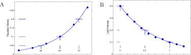
0 20 40 60 80 -1 0 1 2 3 4 5 6 7 8 9 10
Time – Min Depth — layers
Figure 5.5: A. Bacterial population density and ABS=0.022e 0 0315i , which has doubling time of 22 minutes. B. Light depletion and Id = 0.4e~°’ 196d which has a ‘half life’ of 3.5 meters.
In Figure 5.5B is a graph of light intensity decay from Figure 1.10 (repeated in Figure 5.6) and of the Equation 1.15
I d = 0.400 x 0.82 d
Because 0.82 = e ln0 82 = e -°198 ,
I d = 0.400 e -°198d and d 1/2 = = 3.5
1 0.198
Every 3.5 layers of muddy water the light intensity decays by one-half, di/2 is a distance and might be called ‘half depth’ rather than ‘half life.’ ‘Half life’ is the term used for all exponential decay, however, and you are well advised to use it.
Example 5.5.7 Problem. Suppose a patient is prescribed to take 80 mg of Sotolol, a drug that regularizes heart beat, once per day. Sotolol has a half-life in the body of 12 hrs. Compute the daily fluctuations of sotolol.
Solution. Let si be the amount of sotolol in the body at time, t, just before the sotolol pill is taken and sf be the amount of sotolol in the body at time t just after the sotolol pill is taken. Then
s 0 = 0, s+ = 80, s7 = 14 = I 80 = 20.
s+ = st + 80 s t -+i = \s+ = \ (st + 80) = \ si + 20
After some days, si will reach approximate equilibrium, E: si = E and si +l = E. s 0 = 0, s m = | + 20, E = \E+ 20, E = 26.67
Thus, approximately, s t ” = E = 26.67, s+ = s7/ + 80 = E + 80 = 106.67.
so the system oscillates between 26.67 mg and 106.67 mg, a four to one ratio.
You are asked to compare this with taking 40 mg of Sotolol twice per day in Exercise 5.5.6
5.5.4 Semilogarithm and LogLog graphs.
Functions P(t) that satisfy an equation P'(t) = k P(t) may be written P(t) = Poe kt and will satisfy the relation In P(t) = (In Pq) + kt. The graph of In P(t) vs t is a straight line with intercept In P 0 and slope k. Similarly, if P'(t) = —kP(t), in rectilinear coordinates, the graph of
CHAPTER 5. EXPONENTIAL AND LOGARITHMIC FUNCTIONS
248
In P(t) vs t is a straight line with slope —k. A scientist with data t, P(t) that she thinks is exponential may plot the graph of In P(t) vs t. If the graph is linear, then a fit of a line to that data will lead to an exponential relation of the form P(t) = Ae kt or P(t) = Ae~ kt . She may then search for a biological process that would justify a model P'(t) = ±kP(t).
Example 5.5.8 In Section 1.3 we showed the results of an experiment measuring the light decay as a function of depth. The data and a semilog graph of the data are shown in Figure 5.6.
Log (Intensity) = -0.4 – 0.087 Depth
Depth
Figure 5.6: Data and a semilog graph of the data showing experimental results of measuring light decrease with depth of water.
As shown in the figure,
log 10 I d = -0.4 – 0.087 d is a good approximation to the data. Therefore
L = KT 0 4 0 08 ™
= 0.4 x 0.82 d
which is the same result obtained in Section 1.3. As shown in the previous subsection, the relation
I'(d) = -k 1(d) corresponds to a process underlying light depletion in water.
Explore 5.5.8 Do This. In Explore 1.6.1, you were given data for serum penicillin concentration during 30 minutes following a bolus penicillin injection and you may have found that P t = 200 x 0.77 T , where t denotes 5-minute intervals, P t = 200 x 0.978* where t denotes minutes, models the data very well. Additional data for the same experiment is shown in Figure 5.7.
a. On a copy of Figure 5.7 plot the graph of log 10 Pt = log 10 (200 x 0.978′) versus time, t in minutes, for 0 < t < 60.
b. Why is the previous graph a straight line?
c. The two graphs match well for only the first 30 minutes. It is worth a good bit of your time thinking about an alternate model of penicillin pharmacokinetics that would explain the difference after 30 minutes.
CHAPTER 5. EXPONENTIAL AND LOGARITHMIC FUNCTIONS
249
3r
Log 1Q Mezlocillin Concentration
Observed, Serum
t, minutes
0 60 120 180 240 300
Figure 5.7: :
Penicillin concentration following a bolus injection of 2 gm of mezlocillin.
5.5.5 Relative Growth Rates and Allometry.
If y is a positive function of time, the relative growth rate of y is
y(t)
Relative Growth Rate. (5.28)
The relative growth rate of y is sometimes called the fractional growth rate or the logarithmic growth rate.
Definition 5.5.1 Allometry. . Two functions, x and y, of time are said to be allometrically related if there are numbers C and a such that
y{t) = C {x{t)f . (5.29)
If x and y are allometric then
logy = log(Ca; a ) = logC + a logx, (5.30) for any base of log. Therefore if logy is plotted vs logx the graph should be a straight line. Explore 5.5.9 Show that if x and y satisfy Equation 5.30, logy(t) = logC + a \ogx(t), then
y'(t) = x'(t)
y(t) a x(t) ‘
Conclude that if x and y are allometric then the relative growth rate of y is proportional to the relative growth rate of x. m
CHAPTER 5. EXPONENTIAL AND LOGARITHMIC FUNCTIONS
250
Shown in Figure 5.8 is a graph of log 10 of the weight of large mouth bass vs log 10 of their length 9 . The data appear linear and we conclude that the weight is allometric to the length. An equation of a line close to the data is
logy-1.05 _ 2.6-1.05 logx – 2.0 ~ 2.5 – 2.0 :
logy = —5.75 + 3.1 logo;
Then
y
10
-5.75 3.1
The weights of the bass are approximately proportional to the cube of the lengths. This is consistent with the fact that the volume of a cube is equal to the cube of the length of an edge. Many interesting allometric relations are not supported by underlying models, however (Exercises 5.5.29 and 5.5.30).
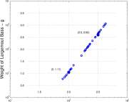
Length of Largemouth Bass – mm
Figure 5.8: Weight vs Length for large mouth bass plotted on a log-log graph.
Exercises for Section 5.5, The derivative equation P’it) = k P(t)
Exercise 5.5.1 Write a solution for each of the following derivative equations. Sketch the graph of the solution. For each, find the doubling time, t^u, or half life, ti/2, which ever is applicable.
Exercise 5.5.2 Write a solution for each of the following derivative equations. Sketch the graph of the solution. For each, find the half life, tu2, which is the time required to ‘move half way toward equilibrium.’
‘Data from Robert Summerfelt, Iowa State University.
CHAPTER 5. EXPONENTIAL AND LOGARITHMIC FUNCTIONS
251
Recall the solution in Example 5.5.5 to solve S'(t) = 15 — 0.055(0-
Exercise 5.5.4 Do Explore 5.5.2. In particular, read the paragraph about the ambiguous use of the variable, t.
Exercise 5.5.5 Suppose a barrel has 100 liters of water and 400 grams of salt and at time t = 0 minutes a stream of water flowing at 5 liters per minute and carrying 3 g/liter of salt starts flowing into the barrel, the barrel is well mixed, and a stream of water and salt leaves the barrel at 5 liters per minute. What is the amount of salt in the barrel t minutes after the flow begins? Draw a candidate solution graph for this problem before computing the solution.
Exercise 5.5.6 In Example 5.5.7 it was shown that in a patient who takes 80 mg of sotolol once per day, the daily fluctuation of sotolol is from 26.7 mg to 106.7 mg. Sotolol has a half-life in the body of 12 hours. What is the fluctuation of sotolol in the body if the patient takes two 40 mg of sotolol at 12 hour intervals in the day? Would you recommend two 40 mg per day rather than one 80 mg pill per day?
Exercise 5.5.7 Suppose it is determined that 30 mg of sotolol is sufficient to control irregular heart beats. What size, X, of sotolol pill should a patient take twice per day to insure that the equilibrium value of sotolol immediately before taking each pill is at least 30 mg?
Exercise 5.5.8 A patient takes 10 mg of Coumadin once per day to reduce the probability that he will experience blood clots. The half-life of Coumadin in the body is 40 hours. What level, H, of Coumadin will be accumulated from previous ingestion of pills and what will be the daily fluctuation of Coumadin in the body.
Exercise 5.5.9 Plot semilog graphs of the data sets in Table Ex. 5.5.9 and decide which ones appear to be approximately exponential. For those that appear to be exponential, find numbers, C and k, so that
P(0 = Ce kt
approximates the the data.
CHAPTER 5. EXPONENTIAL AND LOGARITHMIC FUNCTIONS
252
a.
Table for Exercise 5.5.9 Data sets for Exercise 5.5.9
c.
Exercise 5.5.10 Shown in Table Ex. 5.5.10 data from V. natriegens growth reported in Chapter 1 on page 4. Find numbers, C and k, so that
P(t) = Ce kt
approximates the the data. Use your values of C and k and compute P(0), P(16), P(32), P(48), and P(64) and compare them with the observed values in the Table Ex. 5.5.10.
Table for Exercise 5.5.10 Cell density of V. natriegens measured as light absorbance at
16-minute time increments.
Exercise 5.5.11 In Section 1.3 we found from the discrete model of light extinction,
I d+ i = I d — 0.18/d, that the solution I d+1 — 0.82 I d matched the data for light depletion in Figure 1.11.
Layer
Light Intensity
0
0.400 0.330 0.270 0.216 0.170 0.140 0.124 0.098 0.082 0.065
Light decrease in water is continuous, however. Find a value of k for which the solution to the continuous model, I'(x) = —kl(x), matches the data.
Exercise 5.5.12 In Section 1.6 you may have found that the solution, y = 200 x 0.77*/ 5 , to the difference equation P t+1 — P t = — 0.23 P t , approximates the data for penicillin concentration from Figure 1.18.
Time min
Penicillin
Concentration
0
10 15 20
200 152 118 83 74
Penicillin clearance is continuous, however. Find a value of k for which the solution to P'(t) = —kP(t) matches the data.
CHAPTER 5. EXPONENTIAL AND LOGARITHMIC FUNCTIONS
253
Exercise 5.5.13 David Ho and colleagues 10 published the first study of HIV-1 dynamics within patients following treatment with an inhibitor of HIV-1 protease, ABT-538 which stops infected cells from producing new viral particles. Shown in Exercise Figure 5.5.13A is a graph of plasma viral load before and after ABT-treatment was begun on day 1 for patient number 409 and in Exercise Figure 5.5.13B is a semi-log graph of CD4 cell count following treatment.
a. By what percent is viral load diminished from day-1 to day-12?
b. The line in Figure 5.5.13A has an equation, y = 5.9 — 0.19 a;. Remember that y = log 10 V and x is days. Find V 0 and m so that the graph of V{t) = V 0 e~ mi in semilog coordinates is the line drawn in Exercise Figure 5.5.13A.
c. What is the half-life of the viral load?
d. From the previous step, V'(t) = — 0.43 V(t). Suppose ABT-538 totally eliminates viral production during days 1 to 12. At what rate is the immune system of patient 409 eliminating virus before treatment.
e. Assume that CD4 cell counts increase linearly and the equation in Figure 5.5.13B is y = 9.2 + 15.8 x. At what rate are CD4 cells being produced? Remember that y is CD4 count per mm 3 and there are about 6 x 10 6 mm 3 of blood in the human body.
After about 35 days, the HIV virus mutates into a form resistant to ABT-538 and pre-treatment viral loads soon return. Treatment with a protease inhibitor together with drugs that inhibit the translation of HIV RNA to DNA can decrease viral loads to levels below detection for the duration of treatment.
Figure for Exercise 5.5.13 A. Count of HIV viral load during administration of ABT-538. B.
Count of helper t-cell during the same period. Note that if log 10 (RNA copies per ml) = 4, for example, then RNA copies per ml = 10 4 . See Exercise 5.5.13 Figures adapted by permission at no cost from Macmillan Publishing Group, Ltd. David D. Ho, Avidan U Neumann, Alan S. Perelson,
Wen Chen, John M. Leonard & Martin Markowitz, Nature 373 (1995) 123:127 Copyright 1995
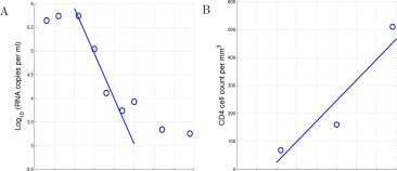
-10 -5 0 5 10 15 20 25 30 -10 -5 0 5 10 15 20 25 30
Day of Treatment Day of Treatment
Exercise 5.5.14 You inject two grams of penicillin into the 6 liter vascular pool of a patient. Plasma circulates through the kidney at the rate of 1.2 liters/minute and the kidneys remove 20 per cent of the penicillin that passes through.
CHAPTER 5. EXPONENTIAL AND LOGARITHMIC FUNCTIONS
254
1. Draw a schematic diagram showing the vascular pool and kidneys as separate entities, an artery leading from the vascular pool to the kidney and a vein leading from the kidney back to the vascular pool.
2. Let P(t) be the amount of penicillin in the vascular pool t minutes after injection of penicillin. What is P(0)?
3. Use Primitive Concept 2 to write an equation for P’.
4. Write a solution to your equation.
Exercise 5.5.15 Suppose a rock sample is found to have 8.02 /ig of 40 K and 7.56 /ig of 40 Ar. What is the age of the rock?
Exercise 5.5.16 Suppose a rock sample is found to have 6.11 mg of 40 K and 0.05 mg of 40 Ar. What is the age of the rock?
Exercise 5.5.17 Rubidium-87 decomposes to strontium-87 with a half-life of 50 x 10 9 years. Fortunately, rubidium and potassium occur in the same rock types and in the same minerals, usually in the ratio of 1 87 Rb atom to approximately 60 0 40 K atoms. Age determined by rubidium-87 to strontium-87 decomposition is an excellent check of 40 K to 40 Ar ages. However, 87 Sr may be lost from the rock or may be present but not derived from 87 Rb so the 87 Rb to 87 Sr age may not be as accurate as the 40 K to 40 Ar age.
a. Suppose a rock sample has 2.5 x 10 11 atoms of 87 Rb and 1.5 x 10 10 atoms of 87 Sr. What is the age of the rock?
b. Suppose a rock sample has 6.4/xg of 87 Rb and 0.01/xg of 87 Sr. What is the age of the rock?
Exercise 5.5.18 A major advancement in archaeology was the development of carbon-14 dating in the 1950’s by an American chemist Willard Libby, for which he received the 1960 Nobel Prize in Chemistry. Carbon-14 develops in the upper atmosphere as neutrons bombard nitrogen, and subsequently combines with oxygen to form carbon dioxide. About 1 in 10 12 CO2 atoms is formed with 14 C in today’s atmosphere. Plants metabolize 14 C0 2 (almost) as readily as 12 C0 2 , and resulting sugars are metabolized equally by animals that eat the plants. Consequently carbon from living material is 1 part in 10 12 carbon-14. Upon death, no additional 14 C is absorbed into the material and 14 C gradually decomposes into nitrogen. Slightly confounding the use of radio carbon dating is the fact that the fraction of atmospheric 14 C02 has not been historically constant at 1 molecule per 10 12 molecules of 12 C0 2 .
Carbon-14 decomposes to nitrogen according to
* 4 C —4 4 N + /T +17 + energy (5.31)
where (5~ denotes an electron and v denotes an antineutrino. One of the neutrons of q 4 C looses an electron and becomes a proton.
Mathematical Model 5.5.5 Carbon-14 decay. The rate of decomposition of g 4 C in a sample is proportional to the size of the sample. One-half of the atoms in a sample will decompose in 5730 years.
CHAPTER 5. EXPONENTIAL AND LOGARITHMIC FUNCTIONS
255
a. Write and solve a derivative equation that will show for a sample of 14 C initially of size Cq what the size will be t years later.
b. In tissue living today, the amount of 14 C in one gram of carbon is approximately 10~ 12 grams. Assume for this problem that the same ratio in living material has persisted for the last 10,000 years. Also assume that upon death the only change in carbon of any form is the decrease in 14 C due to decomposition to nitrogen. Suppose a 100 gram sample of carbon from bone is found to have 3 x 10~ n grams of 14 C What is the age of the sample?
c. Suppose that during the time 10,000 years ago until 2,000 years ago the amount of 14 C in one gram of carbon in living tissue was approximately 1.05 x 10 -12 grams. Suppose a 100 gram sample of carbon from bone is found to have 3 x 10~ n grams of 14 C. What is the age of the sample?
Exercise 5.5.19 Suppose solar radiation striking the ocean surface is 1250 W/m 2 and 20 percent of that energy is reflected by the surface of the ocean. Suppose also that 20 meters below the surface the light intensity is found to be 800 W/m 2 .
a. Write an equation descriptive of the light intensity as a function of depth in the ocean.
b. Suppose a coral species requires 100 W/m 2 light intensity to grow. What is the maximum depth at which that species might be found?
Exercise 5.5.20 In two bodies of water, L\ and L 2) the light intensities h(x) and h(x) as functions of depth x are measured simultaneously and found to be
h(x) = 800 e~ 0Mx and I 2 (x) = 700 e -°05x
Explain the differences in the two formulas in terms of the properties of water in the two bodies.
Exercise 5.5.21 A spectrophotometer is used to measure bacterial cell density in a growth medium. Light is passed through a sample of the medium and the amount of light that is absorbed by the medium is an indicator of cell density. As cell density increases the amount of light absorbed increases. A standard is established by passing a light beam of intensity Iq through a 0.5 cm layer of the growth medium without bacteria and measuring the intensity 1st of the beam emerging from the medium. See Figure Ex. 5.5.21.
Figure for Exercise 5.5.21 Diagram of spectrophotometer. A light beam of intensity Iq enters the standard solution and the intensity 1st of the emerging beam is measured. A light beam of the same intensity I 0 enters the sample solution and the intensity Is m of the emerging beam is
measured. See Exercise 5.5.21.
CHAPTER 5. EXPONENTIAL AND LOGARITHMIC FUNCTIONS
256
Standard
Sample

st

Sm
A light beam of the same intensity Io enters the sample solution and the intensity Is m of the emerging beam is measured.
In the mathematical model of light absorbance (the amount of light absorbed by a layer of water is proportional to the thickness of the layer and to the amount of light entering the layer), the proportionality constant K is a measure of the opacity of the water. Recall that the solution Equation 5.25 is I{x) = Io,e~ Kx .