part0003
- Page ID
- 24589
\( \newcommand{\vecs}[1]{\overset { \scriptstyle \rightharpoonup} {\mathbf{#1}} } \)
\( \newcommand{\vecd}[1]{\overset{-\!-\!\rightharpoonup}{\vphantom{a}\smash {#1}}} \)
\( \newcommand{\id}{\mathrm{id}}\) \( \newcommand{\Span}{\mathrm{span}}\)
( \newcommand{\kernel}{\mathrm{null}\,}\) \( \newcommand{\range}{\mathrm{range}\,}\)
\( \newcommand{\RealPart}{\mathrm{Re}}\) \( \newcommand{\ImaginaryPart}{\mathrm{Im}}\)
\( \newcommand{\Argument}{\mathrm{Arg}}\) \( \newcommand{\norm}[1]{\| #1 \|}\)
\( \newcommand{\inner}[2]{\langle #1, #2 \rangle}\)
\( \newcommand{\Span}{\mathrm{span}}\)
\( \newcommand{\id}{\mathrm{id}}\)
\( \newcommand{\Span}{\mathrm{span}}\)
\( \newcommand{\kernel}{\mathrm{null}\,}\)
\( \newcommand{\range}{\mathrm{range}\,}\)
\( \newcommand{\RealPart}{\mathrm{Re}}\)
\( \newcommand{\ImaginaryPart}{\mathrm{Im}}\)
\( \newcommand{\Argument}{\mathrm{Arg}}\)
\( \newcommand{\norm}[1]{\| #1 \|}\)
\( \newcommand{\inner}[2]{\langle #1, #2 \rangle}\)
\( \newcommand{\Span}{\mathrm{span}}\) \( \newcommand{\AA}{\unicode[.8,0]{x212B}}\)
\( \newcommand{\vectorA}[1]{\vec{#1}} % arrow\)
\( \newcommand{\vectorAt}[1]{\vec{\text{#1}}} % arrow\)
\( \newcommand{\vectorB}[1]{\overset { \scriptstyle \rightharpoonup} {\mathbf{#1}} } \)
\( \newcommand{\vectorC}[1]{\textbf{#1}} \)
\( \newcommand{\vectorD}[1]{\overrightarrow{#1}} \)
\( \newcommand{\vectorDt}[1]{\overrightarrow{\text{#1}}} \)
\( \newcommand{\vectE}[1]{\overset{-\!-\!\rightharpoonup}{\vphantom{a}\smash{\mathbf {#1}}}} \)
\( \newcommand{\vecs}[1]{\overset { \scriptstyle \rightharpoonup} {\mathbf{#1}} } \)
\( \newcommand{\vecd}[1]{\overset{-\!-\!\rightharpoonup}{\vphantom{a}\smash {#1}}} \)
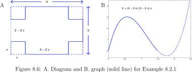
\(\newcommand{\avec}{\mathbf a}\) \(\newcommand{\bvec}{\mathbf b}\) \(\newcommand{\cvec}{\mathbf c}\) \(\newcommand{\dvec}{\mathbf d}\) \(\newcommand{\dtil}{\widetilde{\mathbf d}}\) \(\newcommand{\evec}{\mathbf e}\) \(\newcommand{\fvec}{\mathbf f}\) \(\newcommand{\nvec}{\mathbf n}\) \(\newcommand{\pvec}{\mathbf p}\) \(\newcommand{\qvec}{\mathbf q}\) \(\newcommand{\svec}{\mathbf s}\) \(\newcommand{\tvec}{\mathbf t}\) \(\newcommand{\uvec}{\mathbf u}\) \(\newcommand{\vvec}{\mathbf v}\) \(\newcommand{\wvec}{\mathbf w}\) \(\newcommand{\xvec}{\mathbf x}\) \(\newcommand{\yvec}{\mathbf y}\) \(\newcommand{\zvec}{\mathbf z}\) \(\newcommand{\rvec}{\mathbf r}\) \(\newcommand{\mvec}{\mathbf m}\) \(\newcommand{\zerovec}{\mathbf 0}\) \(\newcommand{\onevec}{\mathbf 1}\) \(\newcommand{\real}{\mathbb R}\) \(\newcommand{\twovec}[2]{\left[\begin{array}{r}#1 \\ #2 \end{array}\right]}\) \(\newcommand{\ctwovec}[2]{\left[\begin{array}{c}#1 \\ #2 \end{array}\right]}\) \(\newcommand{\threevec}[3]{\left[\begin{array}{r}#1 \\ #2 \\ #3 \end{array}\right]}\) \(\newcommand{\cthreevec}[3]{\left[\begin{array}{c}#1 \\ #2 \\ #3 \end{array}\right]}\) \(\newcommand{\fourvec}[4]{\left[\begin{array}{r}#1 \\ #2 \\ #3 \\ #4 \end{array}\right]}\) \(\newcommand{\cfourvec}[4]{\left[\begin{array}{c}#1 \\ #2 \\ #3 \\ #4 \end{array}\right]}\) \(\newcommand{\fivevec}[5]{\left[\begin{array}{r}#1 \\ #2 \\ #3 \\ #4 \\ #5 \\ \end{array}\right]}\) \(\newcommand{\cfivevec}[5]{\left[\begin{array}{c}#1 \\ #2 \\ #3 \\ #4 \\ #5 \\ \end{array}\right]}\) \(\newcommand{\mattwo}[4]{\left[\begin{array}{rr}#1 \amp #2 \\ #3 \amp #4 \\ \end{array}\right]}\) \(\newcommand{\laspan}[1]{\text{Span}\{#1\}}\) \(\newcommand{\bcal}{\cal B}\) \(\newcommand{\ccal}{\cal C}\) \(\newcommand{\scal}{\cal S}\) \(\newcommand{\wcal}{\cal W}\) \(\newcommand{\ecal}{\cal E}\) \(\newcommand{\coords}[2]{\left\{#1\right\}_{#2}}\) \(\newcommand{\gray}[1]{\color{gray}{#1}}\) \(\newcommand{\lgray}[1]{\color{lightgray}{#1}}\) \(\newcommand{\rank}{\operatorname{rank}}\) \(\newcommand{\row}{\text{Row}}\) \(\newcommand{\col}{\text{Col}}\) \(\renewcommand{\row}{\text{Row}}\) \(\newcommand{\nul}{\text{Nul}}\) \(\newcommand{\var}{\text{Var}}\) \(\newcommand{\corr}{\text{corr}}\) \(\newcommand{\len}[1]{\left|#1\right|}\) \(\newcommand{\bbar}{\overline{\bvec}}\) \(\newcommand{\bhat}{\widehat{\bvec}}\) \(\newcommand{\bperp}{\bvec^\perp}\) \(\newcommand{\xhat}{\widehat{\xvec}}\) \(\newcommand{\vhat}{\widehat{\vvec}}\) \(\newcommand{\uhat}{\widehat{\uvec}}\) \(\newcommand{\what}{\widehat{\wvec}}\) \(\newcommand{\Sighat}{\widehat{\Sigma}}\) \(\newcommand{\lt}{<}\) \(\newcommand{\gt}{>}\) \(\newcommand{\amp}{&}\) \(\definecolor{fillinmathshade}{gray}{0.9}\)The bacteria in the sample placed in the spectrophotometer increase the turbidity and therefore the opacity of the solution. Explain why cell density is proportional to
The number In (Ism/1st) is called absorbance.
Exercise 5.5.22 A patient comes into your emergency room and you start a penicillin infusion of 0.2 gms/min into the 6 liter vascular pool. Plasma circulates through the kidney at the rate of 1.2 liters/minute and the kidneys remove 20 per cent of the penicillin that passes through.
a. Draw a schematic diagram showing the vascular pool and kidneys as separate entities, an artery leading from the vascular pool to the kidney and a vein leading from the kidney back to the vascular pool.
b. Let P(t) be the amount of penicillin in the vascular pool t minutes after injection of penicillin. What is P(0)?
c. Use Primitive Concept 2 to write an equation for P’.
d. Compute the solution to your equation and draw the graph of P.
e. The saturation level of penicillin in this problem is critically important to the correct treatment of your patient. Will it be high enough to control the infection you wish to control? If not, what should you do?
f. Suppose your patient has impaired kidney function and that plasma circulates through the kidney at the rate of 0.8 liters per minute and the kidneys remove 15 percent of the penicillin that passes through. What is the saturation level of penicillin in this patient, assuming you administer penicillin the same as before?

CHAPTER 5. EXPONENTIAL AND LOGARITHMIC FUNCTIONS
257
Exercise 5.5.23 An egg is covered by a hen and is at 37° C. The hen leaves the nest and the egg is exposed to 17° C air.
a. Draw a graph representative of the temperature of the egg t minutes after the hen leaves the nest.
Mathematical Model 5.5.6 Egg cooling. During any short time interval while the egg is uncovered, the change in egg temperature is proportional to the length of the time interval and proportional to the difference between the egg temperature and the air temperature.
b. Let T(t) denote the egg temperature t minutes after the hen leaves the nest. Consider a short time interval, [t, t + At], and write an equation for the change in temperature of the egg during the time interval [t, t + At].
c. Argue that as At approaches zero, the terms of your previous equation get close to the terms of
T'(t) = -k(T(t) – 17) (5.32)
d. Assume T(0) = 37 and find an equation for T(t).
e. Suppose it is known that eight minutes after the hen leaves the nest the egg temperature is 35°C. What is fc?
f. Based on that value of k, if the coldest temperature the embryo can tolerate is 32°C, when must the hen return to the nest?
Note: Equation 5.32 is referred to as Newton’s Law of Cooling.
Exercise 5.5.24 Consider the following osmosis experiment in biology laboratory.
Material: A thistle tube, a 1 liter flask, some salt water, and some pure water, a membrane that is impermeable to the salt and is permeable to the water.
The bulb of the thistle tube is filled with salt water, the membrane is place across the open part of the bulb, and the bulb is inverted in a beaker of pure water so that the top of the pure water is at the juncture of the bulb with the stem. See the diagram.
Because of osmotic pressure the pure water will cross the membrane pushing water up the stem of the thistle tube until the increase in pressure inside the bulb due to the water in the stem matches the osmotic pressure across the membrane.
Our problem is to describe the height of the water in the stem as a function of time.
Mathematical Model 5.5.7 Osmotic diffusion across a membrane. The rate at which pure water crosses the membrane is proportional to the osmotic pressure across the membrane minus the pressure due to the water in the stem.
Assume that the volume of the bulb is much larger than the volume of the stem so that the concentration of salt in the thistle tube may be assumed to be constant.
Introduce notation and write a derivative equation with initial condition that will describe the height of the water in the stem as a function of time. Solve your derivative equation.
CHAPTER 5. EXPONENTIAL AND LOGARITHMIC FUNCTIONS
258
Exercise 5.5.25 2 kilos of a fish poison, rotenone, are mixed into a lake which has a volume of 100 x 20 x 2 = 4000 cubic meters. A stream of clean water flows into the lake at a rate of 1000 cubic meters per day. Assume that it mixes immediately throughout the whole lake. Another stream flows out of the lake at a rate of 1000 cubic meters per day.
What is the amount (p t for discrete time or P(t) for continuous time) of poison in the lake at time t days after the poison is applied?
a. Treat the problem as a discrete time problem with one-day time intervals. Solve the difference equation
1000
Po = 2 pt+1 pt = -— pt
b. Let t denote continuous time and P(t) the amount of poison in the lake at time t. Let [t,t + At] denote a short time interval (measured in units of days). An equation for the mathematical model is
Pit)
P(t + At)-P(t) = -^At 1000 Show that the units on the terms of this equation balance.
c. Argue that
P(0) = 2, P'(t) = -0.25 P(f)
d. Compute the solution to this equation.
e. Compare the solution to the discrete time problem, p t , with the solution to the continuous time problem, P(t).
f. For what value of k will the solution, Q(t), to
Q(0) = 2, Q'(t) = kQ(t) satisfy Q(t) = p t , for * = 0,1,2, •••?
g. Which of P(t) and Q(t) most accurately estimates rotenone levels?
h. On what day, t will P(t) = 4g?
Exercise 5.5.26 Continuous version of Chapter Exercise 1.11.7. Atmospheric pressure decreases with increasing altitude. Derive a dynamic equation from the following mathematical model, solve the dynamic equation, and use the data to evaluate the parameters of the solution equation.
Mathematical Model 5.5.8 Mathematical Model of Atmospheric Pressure. Consider a vertical column of air based at sea level and assume that the temperature within the column is constant, equal to 20°C. The pressure at any height is the weight of air in the column above that height divided by the cross sectional area of the column. In a ‘short’ section of the column, by the ideal gas law the the mass of air within the section is proportional to the product of the volume of the section and the pressure within the section (which may be considered constant and equal to the pressure at the bottom of the section). The weight of the air above the lower height is the weight of air in the section plus the weight of air above the upper height.
Sea-level atmospheric pressure is 760 mm Hg and the pressure at 18,000 feet is one-half that at sea level.
CHAPTER 5. EXPONENTIAL AND LOGARITHMIC FUNCTIONS
259
Exercise 5.5.27 When you open a bottle containing a carbonated soft drink, CO2 dissolved in the liquid turns to gas and escapes from the liquid. If left open and undisturbed, the drink goes flat (looses its C0 2 ). Write a mathematical model descriptive of release of carbon dioxide in a carbonated soft drink. From your model, write a derivative equation descriptive of the carbon dioxide content in the liquid minutes after opening the drink.
Exercise 5.5.28 Decompression illness in deep water divers. In the 1800’s technology was developed to supply compressed air to under water divers engaged in construction of bridge supports and underwater tunnels. While at depth those divers worked without unusual physical discomfort. Shortly after ascent to the surface, however, they might experience aching joints, numbness in the limbs, fainting, and possible death. Affected divers tended to walk bent over and were said to have the “bends”.
It was believed that nitrogen absorbed by the tissue at the high pressure below water was expanding during ascent to the surface and causing the difficulty, and that a diver who ascended slowly would be at less risk. The British Navy commissioned physician and mathematician J. S. Haldane 11 to devise a dive protocol to be followed by Navy divers to reduce the risk of decompression illness. Nitrogen flows quickly between the lungs and the plasma but nitrogen exchange between the plasma and other parts of the body (nerve, brain tissue, muscle, fat, joints, liver, bone marrow, for example) is slower and not uniform. Haldane used a simple model for nitrogen exchange between the plasma and the other parts of the body.
Mathematical Model 5.5.9 Nitrogen absorption and release in tissue. The rate at which nitrogen is absorbed by a tissue is proportional to the difference in the partial pressure of nitrogen in the plasma and the partial pressure of nitrogen in the tissue.
Air is 79 percent nitrogen. Assume that the partial pressure of nitrogen in the lungs and the plasma are equal at any depth. At depth d,
a. What is the partial pressure of nitrogen in a diver’s lungs at the surface?
b. Suppose a diver has not dived for a week. What would you expect to be the partial pressure of nitrogen in her tissue?
c. A diver who has not dived for a week quickly descends to 30 meters. What is the nitrogen partial pressure in her lungs after descending to 30 meters?
d. Let N(t) be the partial pressure of nitrogen in a tissue of volume, V, t minutes into the dive. Use the Mathematical Model 5.5.9 Nitrogen absorption and release in tissue and Primitive Concept 2, to write an equation for N’.
e. Check to see whether (k is a proportionality constant)
Plasma pp N 2 = Lung pp N 2

atmospheres.
(5.33)
solves your equation from the previous step.
n J. S. Haldane was the father of J. B. S. Haldane who, along with R. A. Fisher and Scwall Wright developed the field of population genetics.
CHAPTER 5. EXPONENTIAL AND LOGARITHMIC FUNCTIONS
260
f. Assume £ in Equation 5.33 is 0.0693 and d = 30. What is iV(30)?
g. Haldane experimented on goats and concluded that on the ascent to the surface, N(t) should never exceed two times Lung pp N 2 . A diver who had been at depth 30 meters for 30 minutes could ascend to what level and not violate this condition if y — 0.0693?
Haldane supposed that there were five tissues in the body for which £ = 0.139, 0.0693, 0.0347, 0.0173, 0.00924, respectively, and advised that on ascent to the surface, N(t) should never exceed two times pp N 2 in any one of these tissues.
Exercise 5.5.29 E. O. Wilson, a pioneer in study of area-species relations on islands, states in Diversity of Life, p 221, :
“In more exact language, the number of species increases by the area-species equation, S = C A z , where A is the area and S is the number of species. C is a constant and z is a second, biologically interesting constant that depends on the group of organisms (birds, reptiles, grasses). The value of z also depends on whether the archipelago is close to source ares, as in the case of the Indonesian islands, or very remote, as with Hawaii • • • It ranges among faunas and floras around the world from about 0.15 to 0.35.”
Discuss this statement as a potential Mathematical Model.
Exercise 5.5.30 The graph of Figure 5.5.30 showing the number of amphibian and reptile species on Caribbean Islands vs the areas of the islands is a classic example from P. J. Darlington, Zoogeography: The Geographical Distribution of Animals, Wiley, 1957, page 483, Tables 15 and 16.
a. Treat Trinidad as an unexplained outlier (meaning: ignore Trinidad) and find a power law, S = C A z , relating number of species to area for this data.
b. Darlington observes that “• • • within the size range of these islands ■ ■ ■, division of the area by ten divides the amphibian and reptile fauna by two • • •, but this ratio is a very rough approximation, and it might not hold in other situations.” Is your power law consistent with Darlington’s observation?
c. Why might Trinidad (4800 km 2 ) have nearly twice as many reptilian species (80) as Puerto Rico (8700 km 2 ) which has 41 species?
Figure for Exercise 5.5.30 The number of amphibian and reptile species on islands in the Caribbean vs the areas of the islands. The data is from Tables 15 and 16 in P. J. Darlington, Zoogeography: The Geographical Distribution of Animals, Wiley, 1957, page 483.
CHAPTER 5. EXPONENTIAL AND LOGARITHMIC FUNCTIONS
261
in 9 o
03 Q_
tn
_(D
Q. <D k_
re 1°’
c re
0)
.g !c o_ E <
Saba
• ■
Redonda
Trinidad • Puerto Rico
Hispanola
i
Cuba
Jamaica
Montserrat
10 10 10 10 10
Area of Carribbean island (square kilometers)
Exercise 5.5.31 The graph in Figure Ex. 5.5.31 relates surface area to mass of a number of mammals. Assume mammal population densities are constant (each two mammal populations are equally dense), so that the graph also relates surface area to volume.
a. Find an equation relating the surface area, S, of a cube to the volume, V, of the cube.
b. Find an equation relating the surface area, S = 4irr 2 , of a sphere of radius r to the volume, V = |7rr 3 , of the sphere.
c. Find an equation relating the surface area of a mammal to the mass of the mammal, using the graph in Figure Ex. 5.5.31. Ignore the dark dots; they are for beech trees.
d. In what way are the results for the first three parts of this exercise similar?
Figure for Exercise 5.5.31 Graph for Exercise 5.5.31 relating surface area to mass of mammals.
From A. M. Hemmingson, Energy metabolism as related to body size, and its evolution, Rep. Steno Mem. Hosp. (Copenhagen) 9:1-110. With permission from Dr. Peter R. Rossing, Director of Research, Steno Diabetes Center S/A. All rights reserved.
Body surface cm* 3 Kf
iO 5 10* Kf Kf
id
gKf 10 1 Kf Kf 10* 10 s 10 6 10 7 Body weight 1kg it
CHAPTER 5. EXPONENTIAL AND LOGARITHMIC FUNCTIONS
262
Exercise 5.5.32 Body Mass Indices. The Body Mass Index,
rT Mass BMI
Height”
was introduced by Adolphe Quetelet, a French mathematician and statistician in 1869. The Center for Disease Control and Prevention (CDC) notes that BMI is a helpful indicator of overweight and obesity in adults.
From simple allometric considerations, BMI3 = Mass/Height 3 should be approximately a constant, C. If
5M/3 = Mass/Height 3 = C then BMI = Mass/Height 2 = C Height.
so that BMI should increase with height. CDC also states that “• • • women are more likely to have a higher percentage of body fat than men for the same BMI.” If a male and a female both have BMI = 23 and are of average height for their sex (1.77 meters for males and 1.63 meters for females), then
BMI3 for the male
23 L77
13.0 and BMI3 for the female
23 L63
14.1
Thus BMI3 is larger for the female than for the male and may indicate a larger percentage of body fat for the female.
Shown are four Age, and 50th percentile Weight, Height data points for boys and for girls. Compute BMI and BMI3 for the four points and plot the sixteen points on a graph. Which of the two indices, BMI or BMI3, remains relatively constant with age? Data are from the Centers for Disease Control and Prevention, http://www.cdc.gov/growthcharts/data...l/cj41c021.pdf and • • • cj41c022.pdf.
We suggest that BMI3 might be more useful than BMI as an index of body fat. Other indices of body fat that have been suggested include M/H, M 1 / 3 /H, H/M 1 ^ 3 , and cM L2 /# 3 3 . The interested reader should visit the web site cdc.gov/nccdphp/dnpa/bmi and read the references there.
5.6 Exponential and logarithm chain rules.
Suppose an function u(t) has a derivative for all t. Then
CHAPTER 5. EXPONENTIAL AND LOGARITHMIC FUNCTIONS
263
0 u{t)
At)
Exponential Chain Rule. (5.34)
The Exponential Chain Rule is used to prove
1
t
[lnf]’ = and, assuming u is positive,
[lnu(f)]’
u(t)
for t > 0
«'(*)
Logarithm Rule.
Logarithm Chain Rule.
(5.35)
(5.36)
Recall Theorem 4.2.1, The Derivative Requires Continuity. If u(t) is a function and u'(t) exists at t — a
lim u(b) = u(a)
b^a
Proof of the exponential chain rule. We prove the rule for the case the u is an increasing function.
Suppose u(t) has a derivative at t — a and E(t) = e u ^\ To simplify the argument we assume that u(t) is increasing. That is, if a < b, then u(a) < u(b), and, in particular, u(b) — u(a) ^ 0. Then
E'(a) = lim
e u (b) _ e u(a)
b^a b — a
= lim
e «(6) _ e «(a) u (ft) _ u ( a )
f>^a — u(a) 6 — a _ e “( a )
— -u(a) &->a 6 — a
= hm 7^ — x hm —^ — = e w x u (a)
EVig? 0/ Proof. The limit
lim
e «( 6 ) _ e «( a )
3 u(o)
b->a w(6) — -u(a)
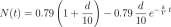
requires some explanation. The graph of y = e x is shown in Figure 5.9. At every point, (x , e x ) of the graph, the slope of the tangent is e x , and specifically at the point (u(a) , e u ^ ) the slope is m = e u(a ). The difference quotient
e u ( b ) _ e «0) u(b) — u(a)
is the slope of a secant to the graph. Because lim u(b) = u(a) the slope of the secant approaches
b^a
the slope of the tangent. Thus
lim
e u ( b ) — e u ( a )
b-*a u(b) — u(a)
Example 5.6.1 Find the derivatives of
P(x) = 200e
-3x
Q(x)
-x 2 /2
CHAPTER 5. EXPONENTIAL AND LOGARITHMIC FUNCTIONS
264
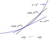
Figure 5.9: Graph of y = e x . Because u'(a) exists, u(b) —> u(a) as b —> a. Therefore the slope of the
secant, ; approaches the slope of the tangent, e
u(a)
Solutions:
P'(x) = [200 e~ 3x ]’ = 200 [e~ 3x ]’ = 200e” 3x [-3s]’ = 200e” 3a; (-3)
Q'(x)
1 e -x 2 /2
_1_
^7T
-a: 2 /2
Logical Identity Constant Factor Rule -s 2 /2]’ Exponential Chain Rule
1 2
e -x 12 (_ x \ Constant Factor, Power Rules
The derivative of P(x) = 200 e 3x also can be computed using the e kt Rule. The e kt rule is a
e fct [Jfet]’ =
special case of the exponential chain rule:
M 11
e kt k.
The derivative of L(t) = Int. The exponential chain rule 5.34 is used to derive the natural logarithm rule, Equation 5.35. In order to use the formula ^e u ^ j = e u ^ u'(t) it is necessary to
know that u'(t) exists. We want to compute [e ln * j and need to know that [hit]’ exists. Our argument for this is shown in Figure 5.10. Also observe that L is increasing so that our argument for the exponential chain rule which assumed that u(t) was increasing is sufficient for this use. Knowing that [hit]’ exists, it is easy to obtain a formula for it.
(5.37)
CHAPTER 5. EXPONENTIAL AND LOGARITHMIC FUNCTIONS
265
E(t) = e l
Figure 5.10: Graphs of E(t) = e* and L(t) = hit and tangents at corresponding points. Because L is the inverse of E, the graph of L is the reflection of the graph of E about the line y = x. Because E has a tangent at (a, b) (that is not horizontal! actually with positive slope), L has a tangent at (b, a) (with positive slope). Therefore L'(b) exists for every positive value of b.
We have now proved the natural logarithm rule, another Primary Formula:

Using the natural logarithm rule and some properties of logarithms we can differentiate y(t) = ln5t + lnt 3 :
y'{t) = [hi5t + lnt 3 ]’
= [ln5 + lnt + 3 1nt]’
= pn5]’ + pnt]’ + [3 Int]’
= 0 +[lnt]’+ [3 lnt]’
= 0 + [lnt]’+ 3 [lnt]’
Symbolic identity Logarithm Prop’s Sum Rule Constant Rule Constant Factor Rule Natural Logarithm Rule
CHAPTER 5. EXPONENTIAL AND LOGARITHMIC FUNCTIONS
266
Example 5.6.2 Logarithm functions to other bases have derivatives, but not as neat as 1/t. We compute L'(t) for L(t) = \og h t where b > 0 and 6^1. Solution.
hit 1 ‘ ln6
i
Info
1 1 Info t
hit]
(0
(»)
(in)
(5.39)
We summarize this as
TTie Logarithm Chain Rule. We now use the Exponential Chain Rule 5.34 to show that if u(t) is a positive increasing function and u'(t) and [lntx(t)]’ exist for all t, then
pnu(f)]’ = ^ [«(*)]’ Proof. By the Exponential Chain Rule and e lnu ^ = u(t),
3 lnu(t)
= [«(*)]’
This is the
e lnMW [lnu(t)]’ = u'(i)
Logarithm Chain Rule
u(t)
(5.41)
Example 5.6.3 Find the derivatives of
a. y = In (V1 – t 2 )
b. y = In f- ^
U + t/
CHAPTER 5. EXPONENTIAL AND LOGARITHMIC FUNCTIONS
267
Solutions:
iln(l-t 2 ) \ [ln(l-t 2 )]’
ll^Kl-i 2 )]’
Logarithm Property
Constant Factor
Generalized Logarithm Rule
Sum, Constant, Constant Factor, and Power Rules
b.
ln(
1 -t T+t
= [ ln(l – J) – m(l + f) ]’ = [ln(l-t)r-[ln(l + Or
-2
Logarithm Property Sum Rule
Generalized Logarithm Rule Sum, Constant, and Power Rules Algebra h
Example 5.6.4 Logarithmic Differentiation. Suppose we are to differentiate
y(t) = (t + 2)(t + l)(t-l) Proceeding indirectly, we first compute the derivative of the natural logarithm of y.
ln(y(0) = ln((f + 2)(f + l)(f-l)) \n(y(t)) = ln(t + 2) + \n(t + 1) + \n(t – 1) [Hy(t))]’ = [ln(t + 2) + ln(t + l) + ln(t- 1)]’
Logical Identity Logarithm Property Logical Identity.
yjt) y ‘^ = TT~2 + 2]’ + fzfj [* + !]’ + fzrj _ 1 ]’ Logarithm chain rule.
[t + C]’ = l. Definition of y.
y'(t) = (f + 2)(f + l)(f-l) + ^ + ^
= (t + l)(t-l) + (* + 2)(i-l) + (f + 2)(t + l) Algebra.
Exercises for Section 5.6, The exponential chain rule and the logarithm chain rule.
CHAPTER 5. EXPONENTIAL AND LOGARITHMIC FUNCTIONS 268 Exercise 5.6.1 Use one rule for each step and identify the rule to differentiate
Exercise 5.6.2 Compute the derivatives of
Exercise 5.6.3 Supply reasons that justify the steps (?) — iiv) in the equations 5.37.
Exercise 5.6.4 Give reasons for the steps (i) — (in) in Equation 5.39 deriving the derivative of the logarithm function L(t) = log 5 t.
Exercise 5.6.5 Find a value for x for which P\x) = 0.
a. Pit) = xe~ x b. Pit) = ex -e~ 2x c. P(t) = x 2 e~ x
Exercise 5.6.6 Use the logarithm chain rule to prove that for all numbers, n:
Power chain rule for all n [ ()” ]’ = n ( -u(t) u'(t)
Assume that u is a positive increasing function and u'(t) exists.
Exercise 5.6.7 Use the logarithmic differentiation to compute y'(t) for
a. y(t) = F b. y(t) = t e c. y(t) = (1 + t 2 f
d. y(t) = t 3 e* e. y(t) = e sillt f. y(t) = t l
Exercise 5.6.8 Use the logarithmic differentiation to compute y\t) for
CHAPTER 5. EXPONENTIAL AND LOGARITHMIC FUNCTIONS
269
5.7 Summary.
The remarkable number e, the exponential function E(t) = e*, and the natural logarithm function L(t) = lnt are the basic material for this chapter. The number e is defined by
lim (1 + c) = = e
It is the only number, b, for which
lim = 1
h^O h
Because \im h ^ 0 (e h — l)/h = 1, the function E(t) = e* has the property that = e*. For any other base, 6 > 0, the exponential function -B(t) = 6* has a derivative, but B'(t) = b t In 6 has the extra factor In6. The natural logarithm function, L(t) = \og e t = lnt also has a simple derivative, 1/t, and its derivative is the simplest among all logarithm functions. For L(t) = log b t, L'(t) = (l/t)/(\nb).
The function E(t) = e kt has the property
E'(t) = e kt k = k E(t)
Many mathematical models of biological and physical systems yield equations of the form
y'(t) = ky(t), and for that reason we frequently use the exponential function e kt to describe natural
phenomena.
When analyzing data thought to be exponential, a semilog graph of the data will often signal whether the data is indeed exponential.
The exponential and logarithm chain rules
e u(t)
1 ‘ ..f-fl / / .N r . / / . \ \ “i / 1
= e
u(t)
u'{t) [In (u(t))}’ = — u'{t)
u(t)
expand the class of functions for which we can compute derivatives, and the logarithm chain rule is used to extend the power chain rule for integer exponents to all values of the exponent.
Exercises for the Summary of Chapter 5. Chapter Exercise 5.7.1 Compute P'(t) for:
a. P(t) = e 5t b. P(t) = Lq5* c. P(t) = e tVl
d. P{t) = e. Pit) = ln(lnt) f. P(t) = e lDt
g. P(t) = 1/(1 + e*) h. P(t) = 1/lni i. P(t) = 1/(1+ e-*)
j. P(t) = (1 + e*) 3 k. P(t) = (e^Y 1. P(t) = InVi
Chapter Exercise 5.7.2 Use the logarithmic differentiation to compute y'(t) for a. y(t) = 10* b. y(t) =
c. y(t) = (t-l) 3 (t 3 -l) d. y(t) = (t-l)(t-2)(t-3)
e. y(t) = u(t)v(t)w(t) f. y(t) = u(t)v(t)
CHAPTER 5. EXPONENTIAL AND LOGARITHMIC FUNCTIONS
270
Chapter Exercise 5.7.3 Use a semilog graph to determine which of the following data sets are exponential.
b.
Chapter Exercise 5.7.4 The function
P(t) =
10 e* 9 + e*
10
9 e-* + 1
is an example of a logistic function. The logistic functions are often is used to describe the growth of populations. Plot the graphs of P{t) and P'(t). P’ and Find at time at which P’ is a maximum. Identify the point on the graph of P corresponding to that time.
Chapter Exercise 5.7.5 A pristine lake of volume 1,000,000 m 3 has a river flowing through it at a rate of 10,000 m 3 per day. A city built beside the river begins dumping 1000 kg of solid waste into the river per day.
1. Write a derivative equation that describes the amount of solid waste in the lake t days after dumping begins.
2. What will be the concentration of solid waste in the lake after one year? Chapter Exercise 5.7.6 Estimate the slope of the tangent to the graph of
y = logio x
at the point (3, log 10 3) correct to three decimal digits.
Chapter Exercise 5.7.7 Use logarithmic differentiation to show that y = te 3t satisfies y” – Qyf + 9y = 0.
Chapter Exercise 5.7.8 Show that for any numbers C\ and C 2 , y = Cie* + C 2 e * satisfies
Chapter 6
Derivatives of Products, Quotients and Compositions of Functions.
6.1 Derivatives of Products and Quotients.
Derivatives of products. We determine the derivative of a function, P, that is a product of two functions, P(t) = u(t) x v(t) in terms of the values of u(t), u'{t), v(t) and v'(t); all four are
CHAPTER 6. DERIVATIVES OF PRODUCTS, QUOTIENTS, COMPOSITIONS
272
required. The formula we obtain is
[«(*)x «(*)]’
u'(t) x v(t)+u(t) X v'(t)
(6.2)
It is not a very intuitive formula. The derivative of a sum of two functions is the sum of the derivatives of the functions. One might expect derivative of the product of two functions to be the product of the derivatives of the two functions. Alas, this is seldom correct, but were it correct your learning of calculus would be notably simplified. The correct formula is used as follows. Let
P(t)
t 3 x e~ 2t
Then with u(t) = t 3 and v(t) = e~ 2t ,
P’it)
x e~ 2t + t 3 x
-2t
3t 2 x e~ 2t +1 3 x e~ 2t x
-2)
A product of functions is useful, for example, in examining the factors affecting total corn production. Total production, P(t), is the product of the number of acres planted, A(t), and the average yield per acre, Y(t). The factors that affect A(t) and Y(t) are distinct. The acres planted, A(t), is affected mostly by government programs and anticipated price of corn; the yield, Y(t), is affected mostly by natural events such as weather and insect prevalence and by improved genetics and farming practices. Government economists often try to maintain total production, P(t), at a fairly constant level, but can affect only A(t), the number of acres planted.
Other instances in which a function is inherently a product of component parts include
1. In simple epidemiological models, the number of newly infected is proportional to the product of the number of infected and the number of susceptible.
2. The rate of a binary chemical reaction A + B — > AB is usually proportional to the product of the concentrations of the two constituents of the reaction.
We prove the following theorem:
Theorem 6.1.1 Suppose u and v are two functions. Then for every number a for which u'(a) and v'{a) exist,
[u{t] x v(t) ]’ t=a = u'(a) x v(a) + u(a) x v'(a)
(6.3)
The proof uses Theorem 4.2.1, The Derivative Requires Continuity, which in symbols is: u(b) — uia) ,
hm = u (a) exists implies that hm uyb) = u{a).
CHAPTER 6. DERIVATIVES OF PRODUCTS, QUOTIENTS, COMPOSITIONS
273
Proof of Theorem 6.1.1.
■ / s / \ i/ ,. u(b) x v(b) — u(a) x via) Mt)xv(t)]’ t=a = hm^ 1 J b _ a y } ^
End of proof.
b^a
u(b) x v(b) – u(a) x v(b) + u(a) x v(b) – u(a) x v(a) b->a b — a
fu(b)—u(a) … , . – u(a)
km I — x v(b) + u(a) x
b->a \ b — a
b — a
fu(b)—u(a) , 7X \ , . ,. v(b)—v(a) = km I — — x v(b) + u(a) x km
b->a \ b — a
b-^a b — a
u(b)—u(a) , . , . ,. v(b)—v(a) km — x via) + u(a) x km
u'(a) x u(a) + u(a) x ?/(a)
fo^a b — a
(0
(«)
(m) (iu)
Explore 6.1.1 In wkick step of Equations 6.4 was Tkeorem 4.2.1, Tke Derivative Requires Continuity, used? ■
(6.4)
Derivatives of quotients. Tke tanx = is tke quotient of two functions, sinx and cosx. Tke logistic function, L(x) = Jt^, used to describe population growtk and ckemical reactions is tke
quotient of two exponential functions. Tkere is a formula for computing tke rate of ckange of quotients:
Theorem 6.1.2 Suppose u and v are functions and u'(a) and v'(a) exist and v(a) ^ 0. Then
At)
UGH! Talk about nonintuitive! Note: v 2 (a) is (v(a)f’.
t—n.
u'(a) x v(a) — u(a) x v'(a) v 2 (a)
(6.5)
CHAPTER 6. DERIVATIVES OF PRODUCTS, QUOTIENTS, COMPOSITIONS
274
Proof of Theorem 6.1.2.
v(t)
t=a
lim
lim
b^a
u(b) u(a) v(b) v(a) b — a
u(b)v(a) — u(a)v(b)
b — a
v(b)v(a)
u(b)v(a) – u(a)v(a) + u(a)v(a) – u(a)v(b)
lim
b— >a
lim
b^a
u(b) — u(a) b — a
v(b)v(a)
v(b) — v(a)
v(a) — u(a)
b — a
v(b)v(a)
( u(b)-u(a)\ v(b)-v(a) lim via) — ula) lim —
\b^a b-a J b^a b – a
^lim v(b)^j v(a)
u'(a) x v(a) — u(a) x v'(a) v(a)v(a)
(i)
(it)
[in
(W
(vi)
(6.6)
End of proof.
Explore 6.1.2 Was Theorem 4.2.1, The Derivative Requires Continuity, used in Equations 6.6? Example 6.1.1 The logistic function and its derivative. The logistic function
PnMe rt
P(t) =
M-P 0 + P 0 e
rt
(6.7)
describes the size of a population of initial size Pq and low density relative growth rate r growing in an environment with limited carrying capacity M. After the function e kt , the logistic function is the most important function in population biology. The graph of a typical logistic curve is shown in Figure 6.1. Obviously, population growth rate, P'(t), is important, and we use the quotient rule to compute it.
CHAPTER 6. DERIVATIVES OF PRODUCTS, QUOTIENTS, COMPOSITIONS
275
P'(t)
P»Me rt M-P 0 + P 0 e rt
P 0 M
-rt
P 0 M
M-P 0 + P 0 e rt . (M-P 0 + P 0 e rt )
M-P 0 + P 0 e
“2
rt
= P 0 M
(M-P 0 + P 0 e rt y
(M-P 0 + P 0 e rt ) e rt xr- e rt (o + P 0 e rt x r ) (M-P 0 + P 0 e rt ) 2
(M -P 0 )e rt r (M-P 0 + P 0 e rt ^
= r
P Q Me rt
)
(M – P 0 )
M-P 0 + P 0 e rt M-P 0 + P 0 e rt rP(t)
M
ii) Hi)
iv)
v)
vi) vii)
(6.8)
Step (v) shows P’. Steps (vi) and (vii) characterize the population growth rate as
P'(t) = rP(t) (
M
(6.9)
The fraction P(t)/M is the density of the population. If the density is small (population size, P(t), is small compared to the environmental carrying capacity, M), the factor 1 — P(t)/M is close to 1 and ‘almost’ P'(t) = rP(t). Almost P'(t)/P(t) = r and for that reason r is called the low density relative growth rate of P. We compare P(t) with the function p(t) which satisfies the simpler equation
p(0) = P o , p'(t)=rp(t)
We know from Section 5.5 that
p(t) = P 0 e rt
The graph of p(t) is shown as the dashed curve in Figure 6.1 where it is seen that p(t) is close to P(t) while P(t) is small.
The number M — P(t) is the unused environment, or the residual environmental capacity. When P(t) is almost as large as M (the density is large), the residual capacity M — P(t) is close to zero and the factor (1 — P(t)/M) is close to zero. From Equation 6.9 the growth rate of the population P'(t) is also close to zero. Equation 6.9 is consistent with:
Mathematical Model 6.1.1 Mathematical model of logistic growth. The growth rate of a population is proportional to the size of the population and is proportional to the residual capacity of the environment in which the population is growing.
We acknowledge that we have reversed the usual role of modeling. We began with a reported solution equation, obtained a derivative equation, and then wrote the model. The steps are reversed with respect to the accepted order in Chapter 1, and with respect to Pierre Verhulst’s development of the model in 1838. The equation is developed in ‘proper’ order in Chapter 17 from Verhulst’s
CHAPTER 6. DERIVATIVES OF PRODUCTS, QUOTIENTS, COMPOSITIONS
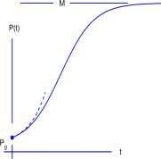
Figure 6.1: The graph of a logistic curve P(t) = P 0 Me rt /(M – P 0 + P 0 e rt ). The dashed curve is the graph of p(t) = Pq e rt showing the close approximation to exponential growth for P(t)/M small (low density).
Mathematical Model of population growth in a limited environment The
growth rate of a population is proportional to the size of the population and to the fraction of the carrying capacity unused by the population.
Example 6.1.2 Examples of computing the derivatives of products and quotients.
a. P(t) = e 2t \nt P'(t)
[e 2t \nt]’
[e 2 *]’ \nt + e 2t [hit]’ e 2t 2 lnt + e 2 ‘ I
b. P(t)
3t-2 4 + t 2
P'(t)
3t-2 4 + t 2
(4 + t 2 ) [3t – 2] / – (3t – 2) [4 + t 2 }’ (4 + t 2 ) 2
(4 + t 2 ) 3 – (3t – 2) (0 + 2t)
(4 + t
12 – 6r
2\2
CHAPTER 6. DERIVATIVES OF PRODUCTS, QUOTIENTS, COMPOSITIONS
277
,2t
c P(t) =
P'(t)
lnt
lnt [e^’-e^lnt]’ (lnt) e 2t 2-e 2 * 1
2i 2t(lnt)-l ‘ t(lnt) 2
Exercises for Section 6.1, Derivatives of Products and Quotients.
Exercise 6.1.1 The word differentiate means ‘find the derivative of. Differentiate
a. P(t) = ^
b. P(t) = e 2lnt
c. P(t) = e t \nt
2 a 2t
A In 2
d. P{t) = t 2 e
e. P(t)
f. P(t)
t
Exercise 6.1.2 Compute P’ for:
a. P(t) = tV
c. P(t)
e. P(t) g- P(t)
i + r
t e* — e*
i. P(t) k. P(t) m. P(t)
Vt lnt
1 lnt
10
.-,0.2*
9 + e
0.2t
g. P(t) = (ef
h. P(t) =
i. P(t) =
3f
It – 1
b. P(t)
d. P(t)
f. P(t)
h. P(t)
j- m
l. P(t)
n. P(t)
= y/t
t + 1 t^T
t lnt-t tV-2te* + 2e*
e* lnt
e (tlnt)
20
1 + 19 e
-o.it
Exercise 6.1.3 Give reasons for steps (i) — (v) in Equations 6.4 proving Theorem 6.1.1, the derivative of a product formula.
Exercise 6.1.4 Give reasons for steps (i) — (vi) in Equations 6.6 proving Theorem 6.1.2, the derivative of a quotient formula.
Exercise 6.1.5 Write an equation that interprets the mathematical model of logistic growth, Mathematical Model 6.1.1 on page 275, and show that it can be written in the form of Equation 6.9.
CHAPTER 6. DERIVATIVES OF PRODUCTS, QUOTIENTS, COMPOSITIONS
278
Exercise 6.1.6 Is there an example of two functions, u(x) and v(x), for which [u(x) x v(x)]’ = u'(x) x v'(x)l
Exercise 6.1.7 Is there an example of two functions, u(x) and v(x), for which
u(x)
v\x)
v'(x) ‘
Exercise 6.1.8 An examination of 1000 people showed that 41 were carriers (heterozygotic) of the gene for cystic fibrosis. Let p be the proportion of all people who are carriers of cystic fibrosis. We can not say with certainty that p = 41/1000. For any number p in [0,1], let L(p) be the likelihood of the event that 41 of 1000 people are carriers of cystic fibrosis given that the probability of being a carrier is p. Then
where ^ * s a constant 1 approximately equal to 1.3 x 10 73 .
a. Compute L'(p).
b. Find the value p of p for which L'(p) = 0 and compute L(p).
The value L{p) is the maximum value of L(p) and p is called the maximum likelihood estimator of p.
Exercise 6.1.9 An examination of 1000 people showed that 41 were carriers (heterozygotic) of the gene for cystic fibrosis. In a second, independent examination of 2000 people, 79 were found to be carriers of cystic fibrosis. Let p be the proportion of all people who are carriers of cystic fibrosis. For any number p in [0,1], let L(p) be the likelihood of finding that 41 of 1000 people in one study and 79 out of 2000 people in a second independent study are carriers of cystic fibrosis given that the probability of being a carrier is p. Then
_, , /1000\ 41 n , 959 /20 00\ 79 n U921 L(P) = ( 41 J V 41 x (1 -p) 959 x I 7g J p 79 x (1 -p) 1921
/1000\ , „ ~ , /2000\ , A _ 14S where I ^ I = 1.3 x 10′ d and I ^ I = 1.4 x 10 i4d are constants.
a. Simplify
b. Compute L'(p).
c. Find the value p of p for which = 0.
The value L(p) is the maximum value of L(p) and p is called the maximum likelihood estimator of p.
Exercise 6.1.10 A bird searches bushes in a field for insects. The total weight of insects found after t minutes of searching a single bush is given by w(t) = ^ grams. Draw a graph of w. From your graph, does it appear that a bird should search a single bush for more than 10 minutes? It takes the bird one minute to move from one bush to another. How long should the bird search each bush in order to harvest the most insects in an hour of feeding?
1 ( ] is the number of r member subsets of a set with n elements, and is equal to
r!(n—r)! ‘
CHAPTER 6. DERIVATIVES OF PRODUCTS, QUOTIENTS, COMPOSITIONS
279
Exercise 6.1.11 Van der Waal’s equation for gasses at high pressure (20 to 1000 atmospheres, say) is
2
( p + ^77^) (V-n*b) = n*R*T (6.10) V 2
where n and R are, respectively, the number of moles and the ideal gas law constant, and a and b are constants specific to the gas under study.
a. Find ^ under the assumption that the volume, V, is constant.
b. Find j£ under the assumption that the temperature, T, is constant. Exercise 6.1.12 Let
P(t) = ^ = u(t) x W))1 Use the product rule and power chain rule to show that
_ u'(t)v(t)-u(t) v\t) F [t) – v\t)
Exercise 6.1.13 Let P(t) = u(t) x v(t). Then
lnP(t) = \n(u(t) x v(t)) = \nu(t) + \nv(t) (6.11)
Compute the derivative of the two sides of Equation 6.11 using the logarithm chain rule and show that
P'(t) =u(t)v'(t)+u'(t)v(t) Exercise 6.1.14 Let P(t) = u{t)/v{t). Then
In P{t) = In (^^j = ln u(t) – In v(t) (6.12)
Compute the derivative of the two sides of Equation 6.12 using the logarithm chain rule and show that
u(t)v'(t) – u'(t)v(t)
P'(t)
v 2 (t)
Exercise 6.1.15 A useful special case of the quotient formula is the reciprocal formula: If u(t) has a derivative and u(t) ^ 0 and
P(t)= ‘
u(t) then
no = ^ At)
Prove the formula using logarithmic differentiation. That is, write
\nP(t) = In (^jj = -lnu(t)
and compute the derivatives of both sides using the logarithm chain rule. We write the formula as
CHAPTER 6. DERIVATIVES OF PRODUCTS, QUOTIENTS, COMPOSITIONS
280
Exercise 6.1.16 Use Equations 6.2 and 6.13 to compute the derivative of
Exercise 6.1.17 Provide reasons for steps (ii), (in), and (iv) in Equations 6.8 computing the derivative of the logistic function. Step (vii) is a hassle. One has to first compute 1 — P(t)/M where P(t) = P 0 Me kt /(M – P 0 + P 0 e kt ). Give it a try.
Exercise 6.1.18 Sketch the graphs of the logistic curve
P 0 Me rt
P(t)
M-P 0 + P 0 e
rt
for
Exercise 6.1.19 For what population size is the growth rate P’ of the logistic population function the greatest? The equation
provides an answer. Observe that y = r p (1 — p/M) = rp — (r/M) p 2 is a quadratic whose graph is a parabola.
The answer to this question is important, for the population size for which P’ is greatest is that population that wildlife managers may wish to maintain to provide maximum growth.
Exercise 6.1.20 Crows on the west coast of Canada feed on a mollusk called a whelk (shown in Figure 6.2) 2 . The crows break the whelk shell to obtain the meat inside by lifting the whelk to a height of about 5 meters and dropping it onto a rock.
Copyright permission to use the figures from Reto Zach’s papers was given by Brill Publishers, PO Box 9000, 2300 PA Leiden, The Netherlands.
Reto Zach (1978,1979) investigated the behavior of crow feeding as an example of decision making while foraging for food, and concluded that crows break the whelk in a manner that minimized their effort (optimal foraging). Crows find whelks in the intertidal zone near the water, carry it towards the land, fly vertically and drop it from a height for breaking. The vertical ascent and drop are repeated until the whelk breaks. Zach made two interesting observations:
2 Reto Zach, Selection and dropping of whelks by northwestern crows, Behaviour 67 (1978), 134-147. Reto Zach, Shell dropping: Decision-making and optimal foraging in northwestern crows, Behaviour 68 (1979), 106-117.
CHAPTER 6. DERIVATIVES OF PRODUCTS, QUOTIENTS, COMPOSITIONS
281
a
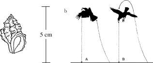
Figure 6.2: a. Schematic drawing of a whelk (Zach, 1978, Figure 1). b. “Flights during dropping. Some crows release whelk at highest point of flight and are unable to see whelk fall (A). Most crows lose some height before dropping but are able to see whelk fall (B).” ( ibid., Fig 6.)
1. The crows fed only on large whelk. When large whelk were not available, crows selected another food source.
2. Consistently the crows dropped the whelk from a height of about 5 meters.
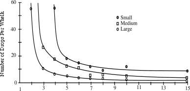
Zach gathered whelks from the intertidal zone, separated them into small, medium, and large categories, and dropped them repeatedly at a given height until they broke. He repeated this at varying heights, and his results are shown in Figure 6.3.
Height of Drop (m)
Figure 6.3: Mean number of drops required for breaking large, medium and small whelks dropped from various heights. Curves fitted by eye. (Zach, 1979, Figure 2.)
We read data from the graph for iV the number of drops required to break a medium sized whelk from a height H and find that the following hyperbola matches the data:
CHAPTER 6. DERIVATIVES OF PRODUCTS, QUOTIENTS, COMPOSITIONS
282
Zach reasoned that the work, W, done to break a whelk by dropping it N times from a height H was equal to N x H. For a medium sized whelk,
W = NxH=(l + 1 )xH H>2. (6.15)
V -0.103 + 0.0389 HJ ~ y ‘
a. Graph Equation 6.15. From your graph, find (approximately) the value of H for which W is a minimum.
b. Compute from Equation 6.15. Find the value H 0 of H for which = 0 and the value W 0 of W corresponding H 0 .
c. Explain why the answers to the two previous parts are equal (or very close).
d. Interpret the quotient Wq/Hq.
e. Data for large whelk (read from an enlargement of Figure 6.3) are shown in Table 6.1. From the graph in Figure 6.3, read the number of drops required to break a large whelk for Height= 2m and Height= 3m and complete the table.
Table 6.1:
Large Size Whelk
f. Find an equation of a hyperbola that matches the data for a large whelk. Note: The number of drops is clearly at least 1, use the equation
N = 1 + ‘
a + bH
and find a and b to match the data. The previous equation can be changed to
N ~ 1 = “TT7) -TT^ = a + bH
a + bH N-l
Therefore a graph of j\f^_ ^ versus H should be approximately linear, and the coefficients of line fit to that data will be good values for a and b. Find a and b.
CHAPTER 6. DERIVATIVES OF PRODUCTS, QUOTIENTS, COMPOSITIONS
283
h. Find the minimum amount of work required to break a large whelk. On average, how many drops does it take to break a large whelk from the optimum height, H Q 7
Summary. The work required to break a medium sized whelk is twice that require to break a large whelk, and the optimum height from which to drop a large whelk is 6.1 meters, reasonably close to the 5.58 meters obtained by Zach.
A similar behavior is observed in sea gulls feeding on mussels. A large mussel broken on the second drop by a gull is shown in Figure 6.4; attached to the large mussel shell is a small mussel that the gull did not bother to break.

Figure 6.4: A large mussel shell broken by a gull on the second drop. Attached to it is a small mussel that the gull did not break. (Photo by JLC)
6.2 The chain rule.
The Power Chain Rule, the Exponential Chain Rule, and the Logarithm Chain Rule have a common pattern and we list all three to show the similarity: If a function, u(t), has derivative then
[u(t) n ]’ = nuity1 x [u(t)}’ Power Chain Rule
= ne u ^ x [u(t)}’ Exponential Chain Rule
e «(*)
In= ^4^j x [«(£)]’ Logarithm Chain Rule
All three of these are of the form
[G(u(t))]’ = G'(u(t)) x [u{t)}’ Chain Rule (6.16)
where
G'(u(t) ) means G'(u), the derivative of G with respect to u.
CHAPTER 6. DERIVATIVES OF PRODUCTS, QUOTIENTS, COMPOSITIONS 284 Consider
G'(u) in the second column is the derivative with respect to u, the independent variable of G, and will often be computed using a Primary Formula.
Example 6.2.1 Compute F'{t) for F(t) = (1 -t 2 f. Let
G(z) = z 3 and u{t) = l-t 2 . Then F(t) = G(u(t)).
G\z) = 3z 2 and [u(t)}’ = -2t, G'(u(t)) = 3(u(t)) 2 = 3(l-t 2 ) 2 ,
and
F'(t) = G'( u(t) ) [«(*)]’ = 3(1- t 2 ) 2 (-2*)
In the form G(-u(t)), may be called the ‘outside’ function and u(t) may be called the inside function. Consider
Theorem 6.2.1 Chain Rule. Suppose G and u are functions that have derivatives and G(u(t) ) is defined for all numbers t. Then G(u(t) ) has a derivative for all t and
[G(u(f))r = C(«(f))x [«(*)]’ (6.17)
Proof: The argument is similar to that for the exponential chain rule. The difference is that we now have a general function G(u) rather than the specific functions e u . We argue only for u an increasing function, and we need Theorem 4.2.1, The Derivative Requires Continuity.
CHAPTER 6. DERIVATIVES OF PRODUCTS, QUOTIENTS, COMPOSITIONS
285
Let F = G o u (F{t) = G{u{t)) for all t).
F(b) – F(a)
F'(a) = lim
b — a
The conclusion that
lim G ( u ( b )) ~ G ( u ( a )) b^a b — a
,. G(u(b))-G(u(a)) ,. u(b)-u(a) lim lim
b^a u(b) — u(a) b^a b — CI
G'{u{a)) u'{a)
G(u(b))-G(u(a))
u{b) – u{a) ^ 0
lim
b-Mi u(b) — u{a)
requires some support.
In Figure 6.5, the slope of the secant is
G'(u(a))
G(u(b)) – G(u(a)) u{b) — u(a)
Because u'(a) exists, u(b) — > u(a) as b —> a. The slope of the secant approaches the slope of the tangent as u(b) —> u(a), and
End of proof.
G(u(b))-G(u(a))
lim ttt = G {u{a)).
b^a u (b) – u(a)
(u(b), G(u(b)))
m = G (u(a))
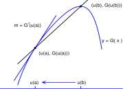
Figure 6.5: Graph of a function y G(u(a) ))/(u(b) – u(a)) -> G'(u(a) ).
As b -> a, (G(u(6))
Example 6.2.2 Repeated use of the chain rule allows computation of derivatives of some quite complex functions.
Problem. Compute the derivative of

t > 1 so that lnt > 0.
Solution. We peel the layers off from the outside. F(t) can be thought of as
F(t) = G (H(K(t))) , where G{z) = e z , H(x) = y/x, and K{t) = lnt
CHAPTER 6. DERIVATIVES OF PRODUCTS, QUOTIENTS, COMPOSITIONS
286
not
f\at
7 lnt
2VhU 1 1
/hit 1 1
2Vm~£*
Extreme Problem. Argh! Compute the derivative of
G(z) = e z , G'{z) = e z H{x) = yfi, H'{x) = ^
K(t) = ]nt, K'(t) = \
F(t) = 1 + Win
l-t T+i
l-t
‘In
1 +t
4 1
l-t
‘In
= 4 1 +Win
1 + t
l-t
T+t
l-t
/In
1 + t
0 +
In
l-t
T+t
4 1 + Win
l-t\ 1
1 + +/,n 1 t
1 + t
l-t \l+t
l-t
ITt
A
4 1 + Win
l-t\ 1
1+t
1 1 (l + t)(-l)-(l-t)l
1 + t
l-t
/In
1+t
l-t T+t
The chain rule is an investment in the future. It does not immediately expand the collection of functions for which we can compute the derivative. To use the chain rule on G(u(t) ) we need G'(u) which requires a Primary derivative formula. The relevant Primary derivative formulas so far developed are the power, exponential and logarithm Primary formulas, for which we have already developed chain rules. In the next chapter, we develop the Primary formula
[sint]’ = cost
Then from the chain rule of this section, we immediately have the chain rule
[sin(w(t))]’ = cos(w(t)) u'{t) Using this we can, for example, compute [sin(7rf) ]’ as
[sin(7rt)]’ = cos(7rt) [nt]’
= COs( Tit ) 7T
Leibnitz notation. The Leibnitz notation makes the chain rule look deceptively simple. For G(u(t)) one has
[(?(«(*))]’= ^ G’Ht)) = d 4 Ht)]> (hl
alt
alu
alt
CHAPTER 6. DERIVATIVES OF PRODUCTS, QUOTIENTS, COMPOSITIONS
287
Then the chain rule is
dG dG du dt du dt
Example 6.2.3 Find ^ for y(t) = (1 + t 4 ) 7 . y(t) is the composition of G(u) = u 7 and u(t) = 1 + t 4 . Then
dG _ d ..7
-j— — -j—u = 7u
du du
6
~dt ~dt K
dG_ = dGdu = 7u 6 x 4t 3 = 7(1 + t 4)6 4t s
Exercises for Section 6.2, The chain rule. Exercise 6.2.1 Use the chain rule to differentiate P(t) for
Exercise 6.2.
Compare your answers for a – c with those of Exercise 6.2.1 a – c.
CHAPTER 6. DERIVATIVES OF PRODUCTS, QUOTIENTS, COMPOSITIONS
288
Exercise 6.2.3 In Chapter 7 we show that [cos(i)]’ = — sin(t). Use this formula and [sint]’ = cost written earlier in this chapter to differentiate:
Exercise 6.2.4 The Doppler effect. You are standing 100 meters south of a straight train track on which a train is traveling from west to east at the speed 30 meters per second. See Figure 6.2.4. Let y(t) be the distance from the train to you and \x(t)\ be the distance from the train to the point on the track nearest you; x(t) is negative when the train is west of the point on the track nearest you.
a. Write y(t) in terms of x(t).
b. Find y'(t) for a time t at which x(t) = —200
c. Time is measured so that x(0) = 0. Write an equation for x(t).
d. Write an equation for y'(t) in terms of t.
e. The whistle from the train projects sound waves at frequency / cycles per second. The frequency, fi, of the sound reaching your ear is
f (+\ 33L4 f c y cles / r18 a
Ut) = 331.4 + y\t) f second ( ° 8)
331.4 m/s is the speed of sound in air. Draw a graph of fh{t) assuming / = 500.
Derivation of Equation 6.18 for the Doppler effect. A sound of frequency / traveling in still air has wave length (331.4 m/s)/(/ cycles/s) = (331.4/f) m/cycle. If the source of the sound is moving at a velocity v with respect to a listener, the wave length of the sound reaching the listener is ((331.4 + v)/f) m/cycle. These waves travel at 331.4 m/sec, and the frequency Jl of these waves reaching the listener is
331.4 m/s _ 331.4 cycles
^ ~ ((331.4 + v)/f) m/cycle ~ 331.4 + v * second
High frequency sound waves may be used to measure the rate of blood flow in an artery. A high frequency sound is introduced on the skin surface above the artery, and the frequency of the waves reflected from the arterial flow is measured. The difference in frequencies emitted and received is used to measure blood velocity.
Figure for Exercise 6.2.4 A train and track with listener location. As drawn,
x(t) is negative
W,
| Train |- x(t)
\
y(t)
E
100
Listener
Exercise 6.2.5 Air is being pumped into a spherical balloon at the rate of 1000 cm 3 /min. At what rate is the radius of the balloon increasing when the volume is 3000 cm 3 ? Note: V(t) = | nr 3 (t).
Exercise 6.2.6 Consider a spherical ice ball that is melting. A reasonable model is: Mathematical Model.
1. The rate at which heat is transferred to the ice ball is proportional to the surface area of the ice ball.
2. The rate at which the ball melts is proportional to the rate at which heat is transferred to the ball.
The volume, V, of a sphere of radius r is and its surface area, S, is Airr 2 . From 1 and 2 we conclude that the rate of change of volume of the ice ball is proportional to the surface area of the ice ball.
a. Write an equation representative of the previous italicized statement.
b. As the ball melts, V, r, and S change with time. Differentiate V(t) = ^7rr 3 (t) to obtain
V'{t) = 4irr 2 (t)r'(t)
c. Use your equation from (a) and the equation from (b) to show that
r'(t) = K where K is a constant
d. Why should K be negative?
e. Because K should be negative, we write
r'(t) = -K
A good candidate for r(t) is
r(t) = —Kt + C where C is a constant
Why?
CHAPTER 6. DERIVATIVES OF PRODUCTS, QUOTIENTS, COMPOSITIONS
290
f. Only discussion included in this part. With r(t) = —KT + C we find that
W{t) = A(l – t/Bf where W[t) is the weight of the ball
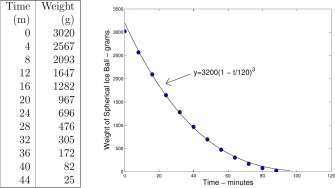
and A and B are constants. In order to test this conclusion, we filled a plastic ball about the size of a volley ball with water and froze it to -14° C (Figure 6.2.6). One end of a chord (knotted) was frozen into the center of the ball and the other end extended outside the ball as a handle. We removed the plastic and placed the ball in a 10° C water bath, held below the surface by a weight attached to the ball. At four minute intervals we removed the ball and weighed it and returned it to the bath. The data from one of these experiments is shown in Table 6.2.6 and a plot of the data and of a cubic, y = 3200(1 — t/120) 3 , is shown in the figure of Table 6.2.6. The cubic looks like a pretty good fit to the data, and we might argue that the data is consistent with our model.
There are some flaws with the fit of the cubic, however. The cubic departs from the data at both ends. y(0) = 3200, but the ball only weighed 3020 g; the cubic is also above the data at the right end.
g. We found that we could fit the data more closely with an equation of the form
W{t) = A{1 -t/100) a where a is closer to 2 than to 3. Find values for A and a. Note:
lnW(t) = In A + aln(l — t/100). Then reasonable estimates of In A and a are the coefficients of a line fit to the graph of lnw(t) versus ln(l — t/100).
h. If the data is not consistent with the model, in what way might the model be deficient?
Figure for Exercise 6.2.6 (h) Pictures of an ice ball used in the experiments described in
Exercise 6.2.6.
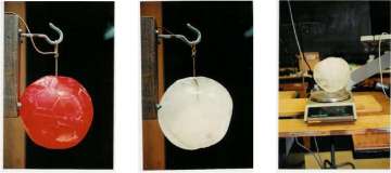
Table for Exercise 6.2.6 Data from an ice ball melt experiment described in Exercise 6.2.6.
CHAPTER 6. DERIVATIVES OF PRODUCTS, QUOTIENTS, COMPOSITIONS
291
6.3 Derivatives of inverse functions.
The inverse of a function was defined in Definition 2.6.2 in Section 2.6.2. The natural logarithm function is the inverse of the exponential function, f(t) = \ft is the inverse of g(t) = t 2 ,t> 0, and f(t) = \/i is the inverse of g(t) = t 3 , are familiar examples. We show here that the derivative of the inverse f~ l of a function f is the reciprocal of the derivative of f, but this phrase has to be explained carefully.
Example 6.3.1 The linear functions
y 1 {x) = l + ^x and y 2 {x) = — + ~z
are each inverses of the other, and their slopes (3/2 and 2/3) are reciprocals of each other.
Explore 6.3.1 Show that in the previous example, y 1 (y 2 (x) ) = x and 2/2(2/1 (x) ) = x.
The crucial point is shown in the graphs of 2/1 and 2/2 in Figure 6.6. Each graph is the image of the other by a reflection about the line y = x. One line contains the points (a, b) and (c, d) and another line contains the points (b, a) and (d,c).
The relation important to us is that their slopes are reciprocals, a general property of a function and its inverse. Specifically,
d—b d—b 1
mi = VTi2 = = —
c — a c — a mi
Example 6.3.2 Figure 6.7 shows the graph of
E(x) = e x and its inverse L(x) = In x
The point (x 3 ,3) has y-coordinate 3. Because E'(x) = E(x) the slope of E at (0:3,3) is 3. The point (3,2 3 ) is the reflection of (x 3 ,3) about y = x and the graph of L has slope 1/3 at (3,x 3 ) because L'(t) = [kit]’ = 1/t. More generally
CHAPTER 6. DERIVATIVES OF PRODUCTS, QUOTIENTS, COMPOSITIONS
292
Figure 6.6: Graphs of y — 1 + (3/2)x and y = —2/3 + (2/3)x; each is the inverse of the other and the slopes, 3/2 and 2/3 are reciprocals.
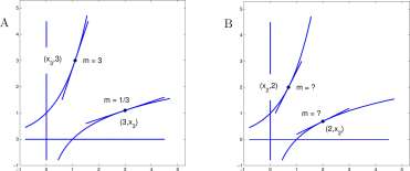
Figure 6.7: Graphs of E(x) = e x and L(x) = In x. Each is the inverse of the other. The point A has coordinates (2, £2) and the slope of L at A is 1/2.
Explore 6.3.2 (a.) Evaluate X3 in Figure 6.7A.
(b.) Evaluate x<± in Figure 6.7B and find the slope at (2:2,2) and at (2,2:2) • ■
The derivative of the inverse of a function. If g is an invertible function that has a nonzero derivative and h is its inverse, then for every number, t, in the domain of g,
If g is an invertible function and h is its inverse, then for every number, t, in the domain of g,
g(h(t))=t We differentiate both sides of this equation.
[g(h(t))}’ = It]’
g'(h(t)) h'(t) = 1 Uses the Chain Rule
hl[t) = g'(h(t)) Assumes 3’W))^0 Explore 6.3.3 Begin with h(g(t) ) = t and show that
9 ‘ (i) = mm
Example 6.3.3 The function, h(t) = \ft, t > 0 is the inverse of the function, g(x) = x 2 , x > 0.
g'(x) = 2x
J. _l_ JL_
[t} ~ 7m) m) ~ 27t’
a result that we obtained directly from the definition of derivative.
Leibnitz notation. The Leibnitz notation for the derivative of the inverse is deceptively simple. Let y = g(x) and x = h(y) be inverses. Then g'(x) = ^ and h'(y) = The equation
j / / \ 1 . dx 1
” W = T7T~i becomes
g'(h(t)) dy ” dy
dx
Exercises for Section 6.3 Derivatives of inverse functions.
Exercise 6.3.1 Find formulas for the inverses of the following functions. See Section 2.6.2 for a method. Then draw the graphs of the function and its inverse. Plot the point listed with each function and find the slope of the function at that point; plot the corresponding point of the inverse and find the slope of the inverse at that corresponding point.
Exercise 6.3.2 The function, h(t) = t 1 ^ is the inverse of the function g(x) = x 3 . Use steps similar to those of Example 6.3.3 to compute h'(t).
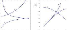
Exercise 6.3.3 The graphs of a function F. its inverse F~ l , and its derivative F’ are shown in each of Figure 6.3.3 (a) and (b).
a. Identify each graph in Figure 6.3.3 (a) as F, F~ l or F’.
b. Identify each graph in Figure 6.3.3 (b) as F, F’ 1 or F’.
Figure for Exercise 6.3.3 Graphs of a function F, -F -1 , and F’. See Exercise 6.3.3.
(a);
3 2
6.4 Summary of Chapter 6.
The thrust of this chapter is to expand your ability to compute derivatives of functions. We have now introduced all of the combination derivative formulas that you will need. Together with the Primary derivative formulas already introduced and two others to be presented in the next chapter, Chapter 7, Derivatives of the Trigonometric Functions, you will be able to compute the derivatives of all of the functions you will meet in ordinary work. The basic formulas that you need are shown below. You need to be able to use them forward and backward. That is, given a function, find its derivative, and given a derivative of a function, identify the function, or several such functions that have that same derivative. The backward process is crucial to the application of the Fundamental Theorem of Calculus, introduced in Chapter 10
The complete list of derivative formulas that you need is:
CHAPTER 6. DERIVATIVES OF PRODUCTS, QUOTIENTS, COMPOSITIONS
295
Chapter Exercise 6.4.1 Differentiate a. p(t) = t A + e 2t
c. P(t)
e. P(t)
g- Pit)
i. P(t)
k. P(t)
m. P(t)
Jit
= e
2I 4
(\ntf
hit t
1
hit
ht 1 -2t-7 t 2 + 1
b. P(t)
d. P(t)
f. P(t)
h. P(t)
j- ^)
1. P(t)
n. P(t)
t 4 e 2t
(t 2 + f) 4 (5t + l) 7 (e 3 * ln2t) 4
t\nt-t
e (lnt)
(t + 2) 2 t 2 + 2
Chapter Exercise 6.4.2 Data from another of the ice ball experiments (see Exercise 6.2.6) are shown in Table 6.4.1.
a. Find a number A so that W(t) = 3200(1 — t/A) 3 is close to the data.
b. Find a number B so that W(t) = 3100(1 – t/B) 2 is close to the data.
c. Which of the two functions is closer to the data?
Close to the data may be defined in at least two ways. For several values of A, compute
SI = \ Wl – 3200(1 -t 1 /Af\ +
CHAPTER 6. DERIVATIVES OF PRODUCTS, QUOTIENTS, COMPOSITIONS
296
S2 = ( Wl – 3200(1 -t l /Aff +
(w 2 – 3200(1 – h/Aff + ■■■ + (w 2 i – 3200(1 – t 2l /Aff
and select the values, Al and A2, of A for which SI and 52, respectively, are the smallest. Then define Wl{t) = 3200(1 – t/Alf and W2(t) = 3200(1 – t/A2) 3 . MATLAB code to do this follows.
Discuss the difference between 51 and S2.
Alter the code to do part b, and then answer part c.
close all;clc;clear t= [0:4:80];
w=[3085 2855 2591 2227 2085 1855 1645 1436 1245 1097 …
908 763 534 513 407 316 216 164 110 88 34] ; AA = [80:1:120];
for i = 1:length(AA)
suml(i) = 0.0; sum2(i) = 0.0; for k = 1:21
suml(i) = suml(i)+ abs((w(k)-3200*(1-t(k)/AA(i))”3)); sum2(i) = sum2(i)+(w(k)-3200*(l-t(k)/AA(i))-3)~2;
end
end
[SI II] = min(suml); A1=AA(I1) [S2 12] = min(sum2); A2=AA(I2)
Wl=3200*(l-t/Al).~3; W2=3200*(l-t/A2).~3;
plot(t,w, ‘x’ ,t,Wl,’o’,t,W2,’+’,’linewidth’,2);
Table for Chapter Exercise 6.4.1 Weight of an ice ball following immersion in 8° C water.
Time m 0 4 8 12 16 20 24 28 32 36 Wt g 3085 2855 2591 2337 2085 1855 1645 1436 1245 1097
Time m 40 44 48 52 56 60 64 68 72 76 80 Wt g 908 763 634 513 407 316 216 164 110 66 34
Chapter 7
Derivatives of the Trigonometric Functions.
7.1 Radian Measure.
Calculus with trigonometric functions is easier when angles are measured in radians. Radian measure of an angle and the trigonometric measures of that angle are all scaled by the length of the radius of a defining circle. For use in calculus you should put your calculator in RADIAN mode.
CHAPTER 7. DERIVATIVES OF THE TRIGONOMETRIC FUNCTIONS
298
The circle in Figure 7.1 has radius 1. For the angle z’ (the angle L AOC) the radian measure, the sine, and the cosine are all dimensionless quantities:
Radian measure of z’ sine of z’ cosine of z’
length of arc AC length of the radius
cm, m, m,
cm, m, m,
length of the segment AB y length of the radius 1
length of the segment OB
length of the radius
x
X
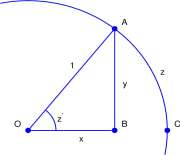
Figure 7.1: A circle with radius 1. The radian measure of the angle z’ is z, the length of the arc AC divided by the length of the radius, 1.
It is obvious 1 from the figure that for z’ in the first quadrant
0 < Length of AB < Length of AC 0 < sin z 1 < z
The inequality, sin z’ < z, is read, ‘the sine of angle z’ is less than z, the radian measure of z’.’ We intentionally blur the distinction between the angle z’ and z, the radian measure of z’, to the point that they are used interchangeably. The inequality
sin z'<z is usually replaced with sinz < z, (7.1)
the sine of z is less than z, where z is a positive number.
The definitions of sin z and cos z for angles that are not accute are extended by use of the unit circle, the circle with center at (0,0) and of radius 1. For z positive, consider the arc of length z counterclockwise along the unit circle from (1,0) to a point, (x,y), in Figure 7.2A. For z negative consider the arc of length \z\ clockwise along the unit circle from (1,0) to a point, (x,y), in Figure 7.2B. In either case
■ y x
smz = – = y cosz = — = x (7.2)
CHAPTER 7. DERIVATIVES OF THE TRIGONOMETRIC FUNCTIONS
299
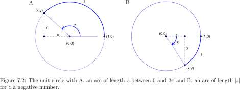
From Figure 7.2B it can be seen that if z is a negative number then
z<sinz<0 (7.3) A single statement that combines Equations 7.1 and 7.3 is written:
|sin^| < \z\ for all numbers z (7-4) We need this inequality for computing [sint] in the next section, and we also need the inequality
7T 7T
\z\ < I tan 21 for — < z < —. (7.5) i i i i 2 2 y J
To see this, for z > 0, examine the circle with radius 1 in Figure 7.3,
—— = AC, and tan ,2 = == = CD.
1 kJkj
We need to show that AC < CD which appears reasonable from the figure, but we present a proof. Proof. The area of the sector of the circle OAC is equal to the area of the whole circle times the
ratio of the length of the arc AC to the circumference of the whole circle. Thus
AC AC
Area of sector OAC = n l 2 x =
2vr x 1 2
The area of the triangle A OCD is
1 fn
Area A OCD = – x 1 x CD =
2 2
The sector OAC is contained in the triangle A OCD so that the area of sector OAC is less than the area of triangle A OCD. Therefore
AC CD
< , AC<CD, and z < tanz.
2
1 Should this not be obvious then reflect the figure about the horizontal line through O, B, and C and let A’ be the image of A under the reflection. The length of the chord A’BA is less than the length of the arc, A’CA (the straight line path is the shortest path between two points).
CHAPTER 7. DERIVATIVES OF THE TRIGONOMETRIC FUNCTIONS
300
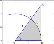
Figure 7.3: The unit circle and an angle z, 0 < z < 7T/2.
An argument for Equation 7.5 for z < 0 can be based on the reflection of Figure 7.3 about the interval OC. End of Proof.
In addition to the basic trigonometric identities, (sin 2 £ + cos 2 £ = 1, tant = suit/ cost, etc.) the double angle trigonometric formulas are critical to this chapter:
sin(A + B) = sin A cos 5 + cos A sin i? cos(A + B) = cos A cos 5 — sin A sin 5. (7-6)
From these you are asked to prove in Exercises 7.1.3
0 fx + y\ . fx-y sin x — sin y = 2 cos sin
2 J V 2
. .’x + y\ . fx-y cos x — cos y = —2 sin —-— sin
Exercises for Section 7.1 Radian Measure. Exercise 7.1.1 For small positive values of z, sinz < z (Equation 7.4), but ‘just barely so’ a. Compute
z — sinz for z — 0.1 for 2 = 0.01 and for 2 = 0.001.
b. Compute
sin z
for z = 0.1 for z = 0.01 and for z = 0.001.
z
c. Note that the slope of the tangent to y — sint at (0,0) is
, sm(0 + h) — sin 0 smh suit L_ n = hm = hm .
J *u /wO h h^O h
What is your best estimate of
[sint]; =0 ?
Exercise 7.1.2 For small positive values of z, z < tanz (Equation 7.5), but ‘just barely so’.
a. Compute
tanz-z for z = 0.01 for z = 0.001 and for z = 0.0001.
b. Compute
for z = 0.01 for z = 0.001 and for z = 0.0001.
c. Note that the slope of the tangent to y — tani at (0,0) is
, tan(0 + h) — tan 0 tank tant L_ n = hm = hm —-—.
H -° h->0 h h^O h
What is your best estimate of
;tant]; =0 ?
Exercise 7.1.3 We need the identities
x + y . x-y sin x —sin y = 2 cos—-— sin—-—
x + y x — y cos a; —cosy = —2 sin—-— sin—-—
in the next two exercises and in the next section. It is unlikely that you remember them from a trigonometry class. We hope you do remember, however, the double angle formulas 7.6,
sin(A + B) = sin A cos B + cos A sin B cos(A + B) = cos A cos B — sin A sin B.
a. Use sm(A + B) — sin A cos B + cos A sin B and the identities, sin(— A) = — sin A and cos(— A) = cos A, to show that
b. Use the equations
to show that
c. Solve for A and B in
sin(A — B) = sin A cos B — cos A sin B
sin(A + B) = sin A cos B + cos A sin B sin(A — B) = sin A cos B — cos A sin B
sin(A + B) – sin(A – B) = 2 cos A sin B (7.7)
A + B = x A-B = y
d. Substitute the values for A + B, A — B, A, and B into Equation 7.7 to obtain
x+y . x-y sin x — sm y = 2 cos —-— sin —-—.
CHAPTER 7. DERIVATIVES OF THE TRIGONOMETRIC FUNCTIONS
e. Use cos(A + B) = cos A cos B — sin A sin B to show that
. fx + y\ . fx-y cos x — cos y = —2 sin ( —-— ) sin
The argument will be similar to the previous steps. Exercise 7.1.4 Use steps (i) — (iv) below to show that at all numbers z,
lim sin(z + h) — sin z,
h~*0
and therefore conclude that the sine function is continuous, (i) Write the trigonometric identity,
fx + y\ . fx-y sin x — sin y — 2 cos [ —-— ) sin
with x = z + h and y = z.
(ii) Justify the inequality in the following statement.
(2z + h>
s\n(z + h) — sin 2; | = 2
cos
h
sin
< 2 x 1 x
h
(iii) Suppose e is a positive number. Find a positive number 5 so that
if \(z + h) — z \ — \ h\ < S then | sin(^ + h) — sin z \ < e
(iv) Is the previous step useful?
Exercise 7.1.5 Use the Inequality 7.4 | sinz | < \z\ and the trigonometric identity,
0 . fx + y\ . fx-y cosx — cosy = —2sin I—-— j sin
to argue that
lim cosf^ + h) — cosz, h-*o y ‘
and therefore conclude that the cosine function is continuous. Hint: Look at the steps {%) – (iv) of Exercise 7.1.4.
7.2 Derivatives of trigonometric functions
We will show that the derivative of the sine function is the cosine function, or
[sint]’ = cost (7.9)
From this formula and the Combination Derivative formulas 6.1 shown at the beginning of Chapter 6, the derivatives of the other five trigonometric functions are easily computed.
CHAPTER 7. DERIVATIVES OF THE TRIGONOMETRIC FUNCTIONS
303
We first show that
[sint]^ =0 = sin'(O) = 1 Assume h is a positive number less than ir/2. We know from Inequalities 7.4 and 7.5 that
sin h < h < tan h
We write
sink < h < tan/i
sin h < 1 < 1 >
h
h sin h
sin h h
<
<
sin h
cos h
1
cos h
> cos h
(ii)
(7.10)
The inequalities
sin h
1 > —— > cos h h
present an opportunity to reason in a rather clever way. We wish to know what
sin h h
approaches as
the positive number h approaches 0 (as h approaches 0 + ). Because cosx is continuous (Exercise 7.1.5) and cosO = 1, cosh approaches 1 as h approaches 0 + . Now we have ‘sandwiched’ between two quantities, 1 and a quantity that approaches 1 as h approaches 0 + . We conclude that also approaches 1 as h approaches 0 + , and illustrate the result in the array:
s in h h
As h -> 0+
1 <
sin h h
< cos h
1 <
<
The argument can be formalized with the e, 5 definition of limit, but we leave it on an intuitive basis.
We have assumed h > 0 in the previous steps. A similar argument can be made for h < 0.
We now know that the slope of the graph of the sine function at (0,0) is 1. It is this result that makes radian measure so useful in calculus. For any other angular measure, the slope of the sine function at 0 is not 1. For example, the sine graph plotted in degrees has slope of 7r/180 at (0,0).
Because of the continuity of the composition of two functions, Equation 4.4, the equation
lim
7i-»0
sin h
h
(7.11)
may take a variety of forms:
sin2/i
lim
h^o 2h
= 1
h
sin —
lim —
h^o h
2
= 1
lim
sin h
= i
We write a general form:
CHAPTER 7. DERIVATIVES OF THE TRIGONOMETRIC FUNCTIONS
304
If 9(h) ^ 0 for h ^ 0 and
lim 9(h) = 0 then lim
sin 9(h) ~9~W
(7.12)
We use
h
sin —
lim—= 1.
a^o ft
2
in the next paragraph. We also use the fact that the cosine function is continuous, Exercise 7.1.5. Now we compute [sint]’ for any t. By Definition 3.22,
r , shift + h) — sint sint = hm .
h^O h
With the trigonometric identity
fx + y\ . (x-y sin x — smy = 2 cos ( —-— ) sin
we get
2
r • . i/ i- sin(t + h) — sint ,.-.
[sintJ = hm j~ (t)
h->0
ft + h + t\ . ft + h-t\
h^o h v 1
iim!!! HHI
2
/ft s
sin
lim cos it + h\ lim £ ‘ (Hi)
h^o \ 2 J h ^o h v ‘
2
‘h\
sin
(7.13)
= cost lim r—— (iv)
2
= cost x 1 = cost (v)
We have now shown that [sint]’ = cost. The derivatives of the other five trigonometric functions are easily computed using the derivative formulas 6.1 shown at the beginning of Chapter 6.
Derivative of the cosine. We will show that
[cost]’ = -sint (7.14)
CHAPTER 7. DERIVATIVES OF THE TRIGONOMETRIC FUNCTIONS
Observe that
71 71 7T
sm(t + —) — sint cos — + cost sin — = sint x 0 + cost x 1 = cost
_ Zi Zi
Therefore
cost = sin(t + —) and [cost]’
sin(t +
7i ,
We use the Chain Rule Equation 6.16
[G(u(t))}’ = G'(u{t)) u'{t) with G{u) = sin-u and u{t) = t + Note that G'(u) = cosw and u'(t) = 1.
7T
[cost] = sin(t H— )
2
7T,
cos(t+ -)
t +
7T
7T,
cos(t + —) X 1
71 71
cos t cos sin t sin —
2 2
— sint
We have established Equation 7.14, [cost]’ = — sint. Derivative of the tangent function. We will show that
[tant]’ = sec 2 t
using
tant
sint
cost
and
sin t ] = cos t and [ cos t] = — sin t
and the quotient rule for derivatives from Equations 6.1,
vu — uv
[tant]’ =
sint” cost.
cost [sint]’ — sint [cost]’
(cost) 2 cost cost — sint (—sint)
cos 2 1 cos 2 1 + sin 2 1
cos 2 t
sec 2 t
In summary we write the formulas
CHAPTER 7. DERIVATIVES OF THE TRIGONOMETRIC FUNCTIONS
306
You are asked to compute [cott]’, [sect]’, and [csct]’ in Exercise 7.2.5.
Example 7.2.1 We illustrate the use of the derivative formulas for sine, cosine, and tangent by computing the derivatives of
a. y = 3sintcost b. y = sin 4 t c. y = ln(tant) d. y = e smt a. [3 sint cost]’ = 3 (sint [cost]’ + [sint]’cost) = 3 (sint (—sint) + cost cost)
= —3 sin 2 1 + 3 cos 2 1
b.
c. [ln(tant)]’
• 4 ±
sin t
= 4(sin 3 t) [sint]’ = 4(sin 3 t) cost.
[(ln(sint)) – (ln(cost))]’
ht ^’-okt M’
sin
cos 2 1 + sin 2 1 cost sint
[ln(sint)]’- [ln(cost)]’
smt COSb cost
sect csct.
„sin t
e s ‘ mt [sint]’
e sint cost
Example 7.2.2 The function F(t) = e~*/ 10 sint is an example of ‘damped oscillation,’ an important type of vibration. Its graph is shown in Figure 7.4. The peaks and valleys of the oscillation are marked by values of t for which F'(t) = 0. We find them by
-t/io
sint
e-*/ 10 [sint]’ +
-t/io
sint
= e
-*/io cos t _ 1-t/io sin t = e -t/io ( CQS t _ 1 gin t
10
10
Now e~*/ 10 > 0 for all t; F'(t) = 0 implies that
cost — — sint = 0, tant = 10, t = (arctan 10) + nn for n an integer.
CHAPTER 7. DERIVATIVES OF THE TRIGONOMETRIC FUNCTIONS
307
-0.8
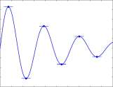
Figure 7.4: Graph of y = e ‘/ 10 sini. The relative high and low points are marked by horizontal tangents and occur at t — arctan 10 + nil for n an integer.
Exercises for Section 7.2 Derivatives of trigonometric functions
Exercise 7.2.1 The difference quotient F(t + h)- F(t)
Make a plot of
approximates F'(t) when h is ‘small.’ h
sm(t + 0.2) — sint n
y = cost and oi <t< 2%.
y 0.2 2 ~ ~
Repeat, using h = 0.05 instead of h = 0.2. Exercise 7.2.2 Compute the derivative of
y(t) = 1 + 2t – 5t 7 + 2e 3t – In 6t + 2 sin t – 3 cos t Exercise 7.2.3 Compute the derivatives of
a. |/ = 2sintcosi b. y = sin 2 1 + cos 2 1 c. y = sect = CQ ^
d. y = cott e. y = In cost f. y = sin 2 1 — cos 2 1
g. y = esc t = , h. y = sec 2 i i. y = e cost
j. y = ln(sect) k. y = e~*sint 1. ?/ = tan 2 t
2t l j.2
m. V = ^qq n. |/= ln(cos 20 t) o. V = J r$y
Exercise 7.2.4 Compute y’ and solve for t in y'(t) = 0. Sketch the graphs and find the highest and the lowest points of the graphs of:
a. y = sin t + cost 0<t<7r b. y = e~*sint 0 < t < n
c. y = \/3 sin t + cos t 0 < t < tv d. y = sin t cos t 0 < t < ir
e. y = e^cost 0 < t < n f. y = e^^cost 0<t<n
Exercise 7.2.5 a. Use cot a; = and the quotient rule to show that
[cot x)’ = — esc 2 x. (7-16)
b. Use secx = CO g X = (cosx) -1 and the power chain rule to show that
[secx] = secxtanx. (7-17)
c. Show that
[ esc x ]’ — — esc x cot x. (7-18)
Exercise 7.2.6 The graphs of y\ = cosh and y 2 = 1 are shown in Figure Ex. 7.2.6. The inequality
sin h
1 < —:— < cos h h
implies that the graph of y = s ^^ , 0 < h < it/ 2 is ‘sandwiched’ between y\ and y 2 – Let F be any function defined on 0 < z < 1 whose graph lies above the graph of y\ and below the graph of y 2 –
1. Draw the graph of one such function, F.
2. What number does F(h) approach as h approaches 0?
Figure for Exercise 7.2.6 Graphs of yi — 1 and y 2 = cos/i. See Exercise 7.2.6.
0.6 –
y 2 = cos h
-0.2 0 0.2 0.4 0.6 0.8 1 1.2 1.4 1.6
h
Exercise 7.2.7 Draw a tangent to the graph of the sine function at the point (0,0) in Figure Ex. 7.2.7. Choose two points of the tangent, measure the coordinates of the two points, and use those coordinates to compute the slope of the tangent and [shit]’ ^ .
Figure for Exercise 7.2.7 Graph of y = sinx. See Exercise 7.2.7.
CHAPTER 7. DERIVATIVES OF THE TRIGONOMETRIC FUNCTIONS
309
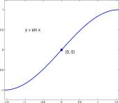
Exercise 7.2.8 Give reasons for steps (i) and (ii) in Equation 7.10 leading to the inequalities
sin h
1 >
> cos/i
It is important that h > 0; why?
Exercise 7.2.9 The derivative of y = cosx is defined by
cos(x + h) — cos x
cosx
lim
/i->0
h
cos(t + 0.2) — cost 02
7T
< t < 2tt.
Make a plot of
y = — sin t and of
Repeat, using h = 0.05 instead of h = 0.2. Exercise 7.2.10 Show that [cost]’ = — sini. To do so, use
cos(t + h) — cost
[cos t\
and the trigonometric identity
cosx — cosy
V 2 J V 2 The steps will be similar to those of Equation 7.13.
Exercise 7.2.11 We have shown that the slope of the graph of the sine function at (0,0) is 1. Use symmetry of the graph of y = sin a; to find the slope of the graph at the point (n, 0). Find an equation of the line tangent to the graph of y = sinx at the point (n, 0). Draw the graph of your line and a graph of y = sin x.
Exercise 7.2.12 Alternate derivation of [cosx]’ = — sinx using implicit differentiation and [sinx]’ = cosx.
Compute the derivatives of both sides of the identity
lim
h^0
. ‘x + y\ . fx-y -2 sin sin
sin 2 x + cos 2 x = 1 and obtain 2 sin x cos x + 2 cos x [cos x] Use the last equation to argue that if cos then
0
cosx
sinx
Exercise 7.2.13 How is the preference in calculus for radian measure of angles for trigonometric functions similar to the preference of the number e as the base of exponential functions?
CHAPTER 7. DERIVATIVES OF THE TRIGONOMETRIC FUNCTIONS
310
7.3 The Chain Rule with trigonometric functions.
The Chain Rule 6.16 states that if G and u are functions that have derivatives and the composition of G with u is well defined then
[G (u(t)) ]’ = G’ («(*)) x [«(*) ]’ = G” («(*)) «'(*)■
With G(u) = sin-u or cos-u or tanw we have
[sin(u(i))]’ = cos(u(*)) x u'(i) = cos(u(*)) u'(t),
[cos (u(t))]’ = — sin(u(i)) u'(t), and
[tan (u(t))]’ = sec 2 (w(t)) u'(i)
Example 7.3.1 For -u(t) = fci where fc is a constant,
[ sin (H) ]’ = cos (kt) x [ fc t ]’ = cos (kt) x fc
Example 7.3.2 With repeated use of the chain rule, derivatives of some rather difficult and exotic functions can be computed. For example, find y’ for
y(t) = In (sin (e cost ))
You may find it curious that y(t) is meaningful for all values of t. In the following, we ‘peel one outside layer at a time’.
y'(t) = [ln(sin(e cost ))] / Outside layer
x [sin(e COB *)] / G(u)=lnu, G'(u) = \
sin
(e cos *)
x cos (e cost ) x [ e cos *]’ G(u) = sin-u, G'(u) = cosu
sin (e cos *)
x cos(e cost ) x e cost x [cost]’ G(u) = e M , G\u) = e u
sin
sin
(e cos *)
/”*” cost \ x cos(e cost ) x e cost x (-sint) G(u) = cos-u, G”(m) = – sin-u [e cos J
= — sint x e cost x cot (e cos *)
Example 7.3.3 We will find in later sections that the dynamics of some physical and biological systems are described by equations similar to
y”(t) + 2y'(t) + 37y(t) = 0. (7.19)
Some of these equations describe functions, y(t), that are defined using sine and cosine functions together with exponential functions. This specific equation has a solution
y (t) = e~*cos6t (7.20)
CHAPTER 7. DERIVATIVES OF THE TRIGONOMETRIC FUNCTIONS
311
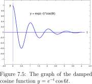
the graph of which is shown in Figure 7.5. The function is called a ‘damped cosine’ function. It is a cosine function whose amplitude is e~* which decreases with time. We show that y(t) = e~* cos6t solves y”(t) + 2y'(t) + 37y(t) = 0.
y ‘(t) = [e _t cost]’
= [ e -‘]’cos6t + e-‘ [cos 6*]’ (i) (7.21)
= (—e~*) cos6t + e~* (—sin6i) x 6 (ii) y”(t) = [~ e ~* cos 6t — 6e~* sin 6t]’
= [—e~ l cos 6£] — 6 [e~* sin 6i] (Hi) = — [e~*]’ cos 6t — e~ l [cos 6t]’
—6 ([e *]’ sin 6t + e~* [sin 6i]’) = e~* cos6t + 6e _ * sin6t + 6e~* sin6t — 36e~* cos6t (v)
= 12e~* sin6i — 35e~* cos6t
We next substitute y(t) = e~ l cos 6i, and the computed values for y'(t) and ?/”(£) into y” + 2y’ + 37?/ and confirm the solution.
V” + 2y’ + 37y
12e _t sin6t — 35e~*cos6t + 2 (—e~* cos6t — 6e~* sin6t) + 37e~*cos6t = (12-2 x 6)e-‘ sin 6t + (-35 – 2 + 37)e~* cos 6t =0
Example 7.3.4 A searchlight is 400 m from a straight beach and rotates at a constant rate once in two minutes. How fast is the beam moving along the beach when the beam is 600 m from the nearest point, A, of the beach to the searchlight.
(iv)
(7.22)
CHAPTER 7. DERIVATIVES OF THE TRIGONOMETRIC FUNCTIONS
312
Searchlight
A
x
600 m
Figure 7.6: Searchlight shining along a beach.
Solution. See Figure 7.6. Let 9 measure the rotation of the light with 9 = 0 when the light is pointing toward A. Let x be the distance from A to the point where the beam strikes the beach. We have
tan(0) =
Both 9 and x are functions of time and we write.
tan0(t) =
x
400
x(t) 400
and differentiate both sides of the equation with respect to t. We get
[tan(f (*))]’ = sec*(9(t))[9(t)}’ =
sec 2 (9(t))9′(t) =
x(t)
400
400
1 400
[x(t)[
At)
Tangent Chain, Constant Factor
The problem is to find x'(t) when x(t) = 600. When x(t) = 600, tan(0(t)) = fjjjj = and
sec 2 {0(t)) = 1 + (|) 2 . The light rotates once every two minutes, so 9′(t) = ^mmute? = 71 radians/minute. Therefore when x(t) = 600,
13
x'(t) = 400 —n meters/minute
Note: Radian is a dimensionless measurement.
Exercises for Section 7.3 The Chain rule with trigonometric functions.
CHAPTER 7. DERIVATIVES OF THE TRIGONOMETRIC FUNCTIONS
313
Exercise 7.3.1 Find y’ for
Exercise 7.3.2 Provide reasons for the differentiation steps (i) — (v) in Equations 7.21 and Equations 7.22.
Exercise 7.3.3 Show that the suggested solutions solve the associated equations.
a. y
b. y
c. y
d. y
e. y f- y
cost cos2t
3 sin t + 2 cos t —3 sin 2t + 5 cos t
e-*
e _< sint
y” + y = o
y” + 4y = 0
y” + y = o
y” + 4y = 0
y” + 2y’ + y = 0
y” + 2y’ + 2y = 0
Exercise 7.3.4 In Example 7.3.4 of the rotating light with beam shining along the beach, where is the motion of the beam along the beach the smallest?
Exercise 7.3.5 A flock of geese is flying toward you on a path that will be directly above you and at a height of 600 meters above you. During a ten second interval, you measure the angles of elevation, 9(t), of the flock three times and obtain the data shown. How fast are the geese flying 2 ?
v
<
Geese
600 m
Observer
6 = Elevation
2 http://north.audubon.org/facts.html#wea shows snow geese migrate 3000 miles at 2952 foot altitude and at an average speed of 50 mph
CHAPTER 7. DERIVATIVES OF THE TRIGONOMETRIC FUNCTIONS
314
Let x(t) denote the horizontal distance from you to the geese. Then
tan = ^ = 600(x(t)y 1 . x(t)
a. Show that
(sec 2 9(t)) x 9\t) = -600 ( x(t) )’ 2 x x'(t) (7.23)
b. The derivative formulas require angles to be measured in radians. Convert the values of 9 in the table to radians.
c. Estimate 9′(5) in radians per second.
d. Compute x(5)
e. Use Equation 7.23 to estimate x'(t) in meters per second for t = 5 seconds. Exercise 7.3.6 In Exercise 7.3.5, the centered difference estimate of 9′(5) is
TT TT
0I{5) = 9m – g(0) = 51 180 q ~ 4 q ° 180 = 0.0192 radians/second.
a. Estimate x’ using this value of 9′.
b. What error in the estimate of x'(t) meters/second might be caused by an error of 0.001 in 0′(5)?
c. With some confidence (and looking at the data), we might argue that
0(5) ~ 0(0) < ff(t , < 0(10)-0(5) 5-0 – U – 10-5
Compute these bounds for #'(5) and use them in similar computations of x'(5) to compute bounds on the estimate of x'(5).
d. Show that an error of size e in 9′ (5) causes an error of 1200 e in x'(5).
Exercise 7.3.7 A piston is linked by a 20 cm tie rod to a crank shaft which has a 5 cm radius of motion (see Figure 7.3.7). Let x(t) be the distance from the rotation center of the crank shaft to the end of the tie rod and 9(t) be the rotation angle of the crank shaft, measured from the line through the centers of the crank shaft and piston. The crank shaft is rotating at 100 revolutions per minute. The goal is to locate the point of the cylinder at which the piston speed is the greatest.
Note: You may prefer to think of this as fly fishing; the crank shaft (rescaled) is your fly rod rotating about your wrist, the tie rod is your fly line, and the piston is a fish.
a. Find an equation relating x(t) and 9{t). You will find the Law of Cosines, c 2 = a 2 + b 2 — 2ab cos C, useful, where a, b, and c are the lengths of the sides of a triangle and C is the angle opposite side c.
b. What is 9′{t)
?
c. What values of x(t) are possible?
d. Differentiate your equation from part (a) to find an equation relating x'(t) to x(t), 9(t), and 6>{t).
e. Evaluate x(t) for 6{t) = 0 + 2tt. Evaluate x'(t) for 6{t) = 0 + 2vr.
f. Evaluate x(t) for 0(t) = | + 2n. Evaluate x'(t) for 6(t) = ^ + 2n.
g. Evaluate x(t) for 8{t) = 1.35 + 2tt. Evaluate x'(t) for 0(t) = 1.35 + 2tt.
T/ie /ast two results may seem a bit surprising, but would be intuitive to fly fishermen and fly fisherwomen. We will return to this problem in Example 8.4-3.
Figure for Exercise 7.3.7 Crank shaft, tie rod, and piston for Exercise 7.3.7.
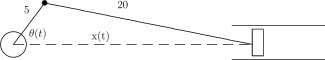
7.4 The Equation y” + u 2 y = 0.
CHAPTER 7. DERIVATIVES OF THE TRIGONOMETRIC FUNCTIONS
316
Harmonic oscillations are ubiquitous in the material world. The sine and cosine functions are called the harmonic functions and at least to first approximation are descriptive of sound waves, light waves, planetary motion, tidal motion, ear drum oscillations, swinging pendula, vibrations of an atom, alternating electrical current, earthquake waves, flutter of a leaf, (the list is quite long).
The most simple equation that applies to oscillating systems in which the resistance to motion is negligible is:
y”(t)+uj 2 y(t)=0 (7.24)
Generally y(t) is the displacement from equilibrium of some measure of the system. The constant uj measures the strength of the force that restores the system to equilibrium. Solutions to the equation are of the form
y(t) = Asm(iut) + Bcos(iut) (7.25)
where A and B are constants that are determined from information about the state of the system at time 0 (for example, y(0) = 1, y'(0) = 0 implies that A = 0 and B = 1). All such functions satisfy y”(t) + uo 2 y(t) = 0. That there are no other solutions follows from the uniqueness of solutions to linear differential equations usually established in differential equation courses. We first establish that if y(t) = Asin(ujt ) then y”(t) + u) 2 y{t) = 0.
y{t) = Asin(ujt)
y'(t) = Acos(ujt) x [cut]’ = A cos( uot ) x uj
ytf(t) = [At; cos (art)]’
= Au(— sin(cut)) x [out]’ = -Auj 2 sin( uot )
It is immediate then that y”{t) + oj 2 y{t) = 0 for
y”(t) + u 2 y{t) = (-A uj 2 sin( ut )) + uj 2 A sin( tut ) = 0
You are asked to show in Exercises 7.4.4 and 7.4.5 that both y(t) = Bcos(ujt) and y(t) = A sin cot +B cos( cot ) solve y”(t) + u 2 y{t) = 0.
It is easy to visualize the motion of a mass suspended on a spring and we begin there. However, the mathematics involved is the same in many other systems; one of the powers of mathematics is that a single mathematical formulation may be descriptive of many systems.
It is shown in beginning physics courses that if y(t) measures the displacement from the rest position of a body of mass m suspended on a spring (see Figure 7.7) with spring constant k, then
my” (t) + ky(t) = 0
. The equation is derived by equating the two forces on the mass,
Newton’s Second Law of Motion Fx = mass x acceleration = m y”
Hooke’s Spring Law F 2 = —k x spring elongation = —k y Fi = F 2 implies that my” = —ky, or my” + ky = 0. (7.26)
E
E
y(t)
A = 2/(0)
Figure 7.7: Oscillation of a mass attached to a spring, a. Relaxed spring with no mass attached, b. A body of mass m is attached and stretches the spring a distance A to an equilibrium position E. c. The body is displaced a distance A below the equilibrium point E and released. y(t) is the displacement of the body from E at time t and is positive when the body is below E.
Assume that the mass is held motionless a distance A below the equilibrium point and at time t — 0 the mass is released. Then
y(0) = A and y'(0) = 0 If we let uj = J— so that uj 2 = — we have
V m m
y(0) = A y'(0) = 0 y”(t) + uj 2 y(t) = 0 (7.27) You will show in Exercise 7.4.4 that the function
y(i) = Acosuot.
satisfies the three conditions of Equations 7.27. It gives a good description of the motion of a body suspended on a spring.
The number u is important. On the time interval [0,2tt/uj], cosut completes one cycle and the position, y(t), of the body progresses from A to —A and back to A. Thus
2tt
PffX
27ry is the period of one oscillation.
One time unit divided by the length of a period of oscillation gives the number of oscillations per unit time and
= — = — \ — is the frequency of oscillations.
27T 27T V m
UJ
CHAPTER 7. DERIVATIVES OF THE TRIGONOMETRIC FUNCTIONS
318
If k/m is ‘large’ (stiff spring or small mass) the period will be ‘short’ and the body oscillates rapidly. If k/m is ‘small’ (weak spring or large mass) the period will be long, the frequency will be low and the body oscillates slowly.
Example 7.4.1 Suppose a body of mass m is suspended from a spring with spring constant k.
1. If m = 20 gm = 0.020 Kg and k = 0.125 Newtons/meter and the initial displacement, y 0 = 5 cm = 0.05 m, then
_ / 0.125 Kg _ , 1 m V 0-020 Kg-m/s 2 /m 1 8
and
y (t) = 0.05cos(2.5t)
The period of oscillation is
_ = __ = 2.51 s. u) 2.51/s
and the frequency of oscillation is approximately
60/2.51 = 23.9 oscillations per minute.
2. If m = 5 gm = 0.005 Kg (one-fourth the previous mass) and k = 0.125 Newtons/meter as before, then the period and frequency of oscillation would be
frn /0.005
Period = 2itJ — — 2n\ — = 2ir x 0.2 = 1.25 seconds per oscillation
V k V 0.125 F
Frequency = —— oscillations per second = 48 oscillations per minute.
Thus one-fourth the mass oscillates twice as fast.
3. If m = 20gm and the spring extends 16 cm when the body is attached to it, then the spring constant, k is
Force 0.02 x 9.8 Kg-Force 1 Newton
k = = x —— = 0.125 Newton/meter
Extension 0.16 meter 9.8 Kg-Force
It is a curious consequence of the previous analysis that the magnitude of the gravitational field, g, is not reflected in the model equation nor in the solution equation. The role of g is to determine the equilibrium location, E. The period and frequency of the oscillations would be the same on the Moon as on Earth.
There are two important omissions in the previous analysis. We have ignored the mass of the spring (which will also be moving) and we have ignored resistance to movement (by the air and in the spring).
CHAPTER 7. DERIVATIVES OF THE TRIGONOMETRIC FUNCTIONS
319
7.4.1 Resistance.
In most systems, the amplitudes of the oscillations decrease with time due to resistance to the movement or friction in the system. Resistance is a force directed opposite to the direction of motion and may be modeled by
Resistance = — r x y'(t) Including the force of resistance with the force of the spring, Equation 7.26 is modified to
my”(t) = -ky(t) – ry'(t)
or
my” (t) +ry'(t) + ky{t) = 0 This is referred to as the equation of damped motion.
(7.28)
Example 7.4.2 Suppose m = 20 gm = 0.020 kg, r = 0.06 Newtons/(meter/sec) and k = 0.125 Newtons/meter. Then the equation of damped motion is
0.02y”(t) + 0.06?/(t) + 0.125y(f) = 0 We show that a solution to this equation is
y (t) = e -1 ” 5 * cos(2f)
(7.29)
At)
y”(t)
e~ 1M cos(2t)
,-1.5t
cos(2t) + e~ 1M [cos(2*)]’
e -1 M (-1.5) cos 2t + e _i 5t (- sin2t) 2
= -1.5e _1 5t cos2t-2e1 5t (siii2t)
1.5e -1 5 * cos2t – 2e” 1 s *(sin2i)
-1.5t/
-1.5 ( [ e~ 1M } cos 2t + e~ 1M [cos 2t}’) – 2 ( [ e~ 1M } sin 2t + e~ 1M fsin 2t}’
= (-1.5) 2 e _i 5t cos 2t + 2(-1.5)(-2)e -1 M sin 2t – 2 2 e~ Lb cos 2t
= -1.75eL5 *cos2t + 6e~ L5 *sin2t Now we set up a table of coefficients and terms of Equation 7.29.
0.02 y”(t) -1.75e15 * cos 2t + 6e1 5 *sin2t
0.06 y'(t) -1.5e _1 5 *cos2i – 2 e 1 5 *sin2t
0.125 y(t)
3 -1.5t
cos 2t
CHAPTER 7. DERIVATIVES OF THE TRIGONOMETRIC FUNCTIONS
320
After substitution into Equation 7.29 the coefficients of e L5i cos 2t and e L5t sin 2t are
0.02 x (-1.75) + 0.06 x (-1.5) + 0.f25 x f = 0.0 and 0.02 x 6 + 0.06 x (-2) = 0.0
so
y (t) = e~ L5t cos(2t) solves 0.02/ (t) + 0My'{t) + 0.125y(t) = 0.
In the previous problem, the resistance, r = 0.06 was selected to make the numbers in the solution (-1.5 and 2) reasonably tractable. The resistance, r = 0.06 is so great, however, that the oscillations are imperceptable after only two or three oscillations, as illustrated in Figure 7.8A.
If r = 0.002 then the solution is
y (t) = e-° At cos(V6.2475t) = eai *cos(2.4995t)
and is shown in Figure 7.8B.
A
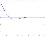
B
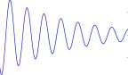
Figure 7.8: A. Graph of y(t) = e~ 1M cos(2t). B. Graph of y(t) = e -0 1 * cos(2.4995t).
If the resistance in a vibrating system is quite large (system is buried in molasses), the system may not vibrate at all but may just ooze back to equilibrium after a displacement. Equation 7.28, my”(t) + ry’it) + ky(t) = 0, may be written (divide by m)
y”{t) + 2by'(t) + cy(t) = 0, where b = r/(2m) and c = k/rn. The solutions to Equation 7.30 are Bolts of Lightning
if b 2 -c>0
(7.30)
1- y(t)
2. y(t)
3. y(t)
ebt {A + Bt) if 6 2 -c = 0
v^Ft if J 2 -c<0,
A e ht sin sjc — bH + B e ■” <•< >s
-bt
(7.31)
where A and B are constants determined by y(0) and y'(0). All three can be shown by substitution to solve Equation 7.30.
CHAPTER 7. DERIVATIVES OF THE TRIGONOMETRIC FUNCTIONS
321
The condition for overdamping, no oscillation in the system, is r 2 > 4km – the square of the resistance is greater than 4 times the spring constant times the mass.
If the formulas above remind you of the roots to a quadratic polynomial, it is not an accident; the connection is shown in Exercise 7.4.6.
The body suspended on a spring is easy to experiment with and typifies many oscillations that occur throughout nature. Other mechanical systems that have similar oscillations include the swinging pendulum and a rotating disc (as in the flywheel of a watch). Less apparent oscillating systems include diatomic molecules in which the distance between the two atoms oscillates very rapidly but can be approximated with the harmonic equations. In the next section we will give a simplified biological example of oscillations in predator-prey systems.
Exercises for Section 7.4, The Equation y” + uo 2 y = 0.
Exercise 7.4.1 Show that the proposed solutions satisfy the equations and initial conditions.
Solution Derivative Equation Initial conditions
CHAPTER 7. DERIVATIVES OF THE TRIGONOMETRIC FUNCTIONS
322
i. y (t) = e^sint y” + 2y’ + 2y = 0 y(0) = 0
y'(0) = 1
j. y (t) = e0At cos2t y” + 0.2y’ + A.Oly = 0 y(0) = 1
y'(0) = -0.1
k. y(t) = y” + 0.2y’ + AMy = 0 y(0) = 2
e-°u (0.1sin2t + 2cos2t) y'(0) = 0
Exercise 7.4.2 Find a number u so that the proposed solution satisfies the derivative equation.
Solution Derivative equation
a. y(t) = 3cos5t yff + u 2 y = 0
b. y{t) = 2 sin 3t + 5 cos 3t ytt + u 2 y = 0
c. y(t) = —4cos7rt y!! + uj 2 y = 0
d. y{t) = 3e~*cos5t yf/ + 2y’ + oo 2 y = 0
e. y(t) = -4e” 2 *sin3t yft + Ay’ + u 2 y = 0
Exercise 7.4.3 Find a number k so that the proposed solution satisfies the derivative equation.
Solution Derivative equation
Exercise 7.4.4 Show that if B and uj are constants and y(t) = Bcos(ut), then
y(0) = B y'(0) = 0 and y”(t) + u 2 y(t) = 0.
Exercise 7.4.5 Show that if A, B and u; are constants and y(t) = Asm(ut) + B cos(ut), then
y (0) = B y'(0) = ujA and y”(t) + u 2 y(t) = 0.
Exercise 7.4.6 Recall Equation 7.30
y”(t) + 2by'(t) + cy(t) = 0
and suppose that m is a number such that y(t) = e mt solves this equation. Compute y'(t) = [e mt ]’ and y”(t). Substitute them into the equation, observe that e mt is never zero, and conclude that
CHAPTER 7. DERIVATIVES OF THE TRIGONOMETRIC FUNCTIONS
323
From this we conclude that
y(t) is either e (-b+VB^)t QT e{ b -VW^c)t
Both are solutions to Equation 7.30. If b 2 — c > 0, these are the terms in solution 1 of
Equations 7.31. The exact condition b 2 — c seldom occurs in nature. The issue for b 2 — c < 0 is how
to interpret _ _
where i = y/—l. Warning: Incoming Bolt from the Blue. The answer is that 3
This suggests (to some people at least) that
y (t) = e~ bt cos Vc-b 2 t + ie~ bt sin Vc-b 2 t
is a solution to Equation 7.30 BANG. Because Equation 7.30 has real number coefficients, some people think that the real and imaginary parts of y(t) should each solve Equation 7.30. They do, and with tenacity you can show that they do. See Exercise 7.4.7.
Exercise 7.4.7 At least, show that
y (t) = ebt cos(Vc-6 2 t)
solves
y”(t) + 2by'(t) + cy(t) = 0 for c – b 2 > 0
Exercise 7.4.8 The complete solution to Exercise 7.4.7 is given in the Solutions Section on the web. Try your hand with showing that
y (t) = ebt sm(V7^¥ t)
solves
y”(t) + 2by'(t) + cy(t) = 0 for c – b 2 > 0 for 6=1, c = 2. Get a big piece of paper.
7.5 Elementary predator-prey oscillation.
Predator-prey systems are commonly cited examples of periodic oscillation in biology. Data from trapping records of the snowshoe hare and lynx gathered by trappers and sold to the Hudson Bay Company are among the most popular first introduction. Shown in Figure 7.9 is a graph showing the numbers of pelts purchased by the Hudson Bay Company for the years 1845 to 1935, and in Table 7.1 are some values read from the graph. 4
3 We will try to convince you that this is reasonable in Chapter 12.
4 Recent studies also demonstrate the fluctuations as shown on the web site http://lynx.uio.no/catfolk/sp-accts.htm. “Lynx density fluctuates dramatically with the hare cycle (Breitenmoscr et al. Oikos 66 (1993), pp. 551-554). An ongoing long-term study of an unexploited population in good quality habitat in the Yukon found densities of 2.8 individuals (including kittens) per 100 km2 during the hare low, and 37.2 per 100 km2 during the peak (G. Mowat and B. Slough, unpubl. data).”
CHAPTER 7. DERIVATIVES OF THE TRIGONOMETRIC FUNCTIONS
324
1 60
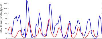
1 S50 1 S60 1870 1SSO 1890 1900 1910 1920 1930
Years
Figure 7.9: Graph of snowshoe shoe hare and lynx pelts purchased by the Hudson Bay company for the years 1845 to 1945. Data read from Figures 3 (hare) and 16 (lynx) of D. A. MacLulich, Fluctuations in the number of varying hare, University of Toronto Studies, Biological Sciences, No. 43, 1937.
Table 7.1: Part of the data read from D. A. MacLulich, ibid.
Hare Lynx Data
Explore 7.5.1 Do this. Complete the phase graph shown in Figure 7.5.1 using data from Table 7.1. Plot the points for the years 1915, 1917, and 1919 and draw the missing lines. ■
Explore Figure 7.5.1 Phase graph axes for hare and lynx data.
X
£
Q_
’27 ’25
’29
’13
‘ ’23
/
• 11
’09
’21
’31
0 20 40 60 80
Hare Pelts Harvested (thousands)
CHAPTER 7. DERIVATIVES OF THE TRIGONOMETRIC FUNCTIONS
325
The phase graph that you just drew is a good way to display the interaction between two populations. You should see a general counter clockwise direction to the graph. When you are in the right-most portion of the region with large hare population, the lynx population is increasing (the curve goes up). As you get to the upper right corner the lynx population has increased sufficiently that the hare population decreases (the curve goes to the left). And the pattern continues. We will return to the lynx-hare data in Exercise 7.5.6 and find that there are exceptions to this pattern in the data.
Nils Chr. Stenseth, Wilhelm Falck, Ottar N. Bjrnstad, and Charles J. Krebs, argue in Population regulation in snowshoe hare and Canadian lynx: Asymmetric food web configurations between hare and lynx, Proc. Nat. Acad. Sci. USA 95 (1995), 5147-5152, that
” • • -the classic view of a symmetric hare — lynx interaction is too simplistic. Specifically, we argue that the classic food chain structure is inappropriate: the hare is influenced by many predators other than the lynx, and the lynx is primarily influenced by the snowshoe hare.”
A Predator-Prey Model. Assume that there are two populations that interact as predator and prey in a reasonably isolated environment. Let U(t) denote the number of prey and V(t) denote the number of predators, and assume there are equilibrium values, U e and V e , so that U e prey would provide enough food for V e predators to just maintain their numbers (predator birth rate = predator death rate) and V e predators would just balance the often excess birth rate of the prey (prey birth rate = prey death rate).
Shown in Figure 7.10 is an axis system where the horizontal axis is U(t) and the vertical axis is V(t). An equilibrium point, (U e , V e ), is plotted. If for some time, t, the populations are not at equilibrium, we let
u(t) v(t)
U(t) V(t)
measure the departures from equilibrium.
V(t), Predator
(U(t),V(t))
v(t)

j
u(t)
/ /
X
U(t), Prey
Figure 7.10: Axes for a predator prey phase graph. The gaps in the axes allow u(t) to be small compared to U e and v(t) to be small compared to V e .
CHAPTER 7. DERIVATIVES OF THE TRIGONOMETRIC FUNCTIONS
326
Suppose the populations U(t) and V(t) are in equilibrium and the predator population increases (perhaps some predators immigrate into the system). The excess predators would increase capture of prey, and we could expect the prey population to decrease. Alternatively, if the prey should become more numerous, the predators would have a greater food supply and their numbers may increase.
Mathematical Model 7.5.1 For small deviations, u(t) and v(t), from equilibrium, we assume that
1. The rate of prey population decrease, —U'(t), is proportional to the excess predator population, v(t).
2. The rate of predator population increase, V'(t), is proportional to the excess prey population, u(t).
Thus from Part 1 we write
-U'(t) = ax v(t) or U'{t) = -a v(t)
By the model, if the predator population exceeds equilibrium, V(t) > V e (v(t) > 0), then U'(t) < 0 and the prey population will decrease. However, if the predator population is less than normal, V(t) < V e (v(t) < 0), then U'(t) > 0 and the prey population increases. For this model, both populations must be assumed to be close to equilibrium. For example, a prey population greatly exceeding equilibrium, U e might support a predator population slightly above equilibrium Ve and still grow.
Because u(t) = U(t) – U e , U(t) = U e + u(t) and
U'(t) = u'(t).
We write
u'(t) = -a v(t)
Similarly,
v ‘(t) = b u(t)
Explore 7.5.2 Show that Part 2 of the Mathematical Model 7.5.1 leads to the equation
v ‘(t) = bu(t)
where b is a proportionality constant. ■ The two equations
u'(t) = -av{t) v ‘{t) = bu{t)
describe the dynamics of the predator – prey populations. There are two unknown functions, u and v, and the equations are linked, because u’ is related to v and v’ is related to u. There is a general
CHAPTER 7. DERIVATIVES OF THE TRIGONOMETRIC FUNCTIONS
327
procedure to obtain a single equation involving only u, as follows:
u'(t) = —av(t) First Original Equation.
[u'(t)}’ = [—av(t)]’ Differentiate First Eq.
u “(t) = -av'(t)
u”{t) = —a{bu{t)) Substitute Second Eq.
u”(t) + (ab)u(t) = 0 Now we let uo = \fab so that uo 2 = a b and write
u”(t) + uo 2 u(t) = 0 (7.32)
and see that it is equivalent to the dynamic equation in Equations 7.27. To complete the analogy, we need -u(O) and -u'(O).
Suppose we have a predator-prey pair of populations and because of some disturbance to the environment (rain, cold, or fire, for example) at a time, t = 0, the populations are at (U 0 , V 0 ), close to but different from the equilibrium values (U e , V e ). Let the departures from equilibrium be
u 0 = U 0 – U e and v 0 = V 0 – V e
Then clearly we will use -u(O) = uq. Also, from u'{t) = —av(t) we will get w'(0) = — av(0) = —at> 0 . Thus we have the complete system
u(0) = u 0 u'(0) = -a v 0 u”(t) + uo 2 u(t) = 0 (7.33)
From Equation 7.24 y”(t) + uo 2 y(t) = 0, and its solution, Equation 7.25, y(t) = Asin(ujt) + B cos(ut), we conclude that u(t) will be of the form
u{t) = Asm(ut) + B cos(ujt)
where A and B are to be determined. Observe that
u'(t) = Aoj cos(c<jt) — B uo sin(c<jt)
Now,
u(0) = Asin{uj ■ 0) + B cos{u ■ 0) = A ■ 0 + B ■ 1 = B u'(0) = Au cos(uj ■ 0) – Busm(u ■ 0) = Auo ■ I – B uo ■ 0 = Auo
It follows that
B = uo and Au = — avo, so that A — t> 0
and the solution is
u(t) = vo sin(u;t) + uq cos (cut)
Remembering that uo = Vab we may write
CHAPTER 7. DERIVATIVES OF THE TRIGONOMETRIC FUNCTIONS
328
u(t)
a b
Vq sin( y/ab t) + u 0 cos( \fab t)
= —Vq J ^ sin(va6 t) + u 0 cos(Vafe t) Explore 7.5.3 Also remember the first equation, u'(t) = —av(t) and show that
v(t) = Vq cos( v a b t) + uq \ — sin( Vabt)
V a
(7.34)
(7.35)
A little trigonometry It often happens that a periodic oscillation is the sum of two oscillations of the same frequency as in Equations 7.34 and 7.35. When that happens, the two can be combined into a single sine function. Suppose F(t) = Asm(u}t) + _Bcos(u;t) where A, B, and uo are numbers.
Let 0 be an angle such that
A
COS (i
Then
Sllli
VA 2 + B 2 B
x/A 2 + B 2
F(t) = Asm(ut) + Bcos(u;t) = VA 2 + B 2
sm(uxt)
B
t VA 2 + B 2 VA 2 + B 2
V A 2 + B 2 (cos 4>sm(ut) + sin (j)cos(ujt))
cos(uit)
= \lA 2 + B 2 sm(ujt + 4>) The last step uses sin(a + (3) = sin a cos j3 + cos a sin j3.
Exercises for Section 7.5, Elementary predator-prey oscillation.
Exercise 7.5.1 Suppose that a = b = 1 and uq = 3 and vq = 4 in the prey equation 7.34 so that
u (t) = -4sin(t) +3cos(t).
(uq and v 0 are ‘small’ disturbances. We might suppose, for example, that the equilibrium populations are U e = 300, V e = 200, with 3 and 4 ‘small’ with respect to 300 and 200).
a. Sketch the graph of u(t) = — 4sin(t) + 3cos(t).
b. Let (j) (the Greek letter phi) denote the angle between 0 and 2n whose sine is | and whose cosine is Show that
u(t) = 5 (cos <fi sin t + sin 0 cost) = 5 sin(t + <fi)
c. Plot the graph of 5sin(t + 0) and compare it with the graph of —4 sint + 3cost.
Exercise 7.5.2 Compare Equation 7.34, u(t) = —v 0 sm(s/ab t) + Uq cos{\fab t) for the two
cases:
Case 1: a = b = 1 and u 0 = 3 and v 0 — 4 (in the previous problem). Case 2: a = 4, b = 1 and Uo = 3 and v 0 = 4
What is the biological interpretation of the change from a = 1 to a = 4?
Exercise 7.5.3 a. Find the formula for the predator population Equation 7.35 using the parameters, a = b = l,u 0 = 3 and v 0 = 4.
b. Let ip (Greek letter psi) be the angle between 0 and 2-7T for which
cos-0 = – and sin-0 = -5 5
and show that
v(t) = 5sin(t + ip)
Exercise 7.5.4 Develop the predator harmonic equation.
a. Examine the steps leading to Equations 7.33 and show that
v{0) = v 0 v'{0) = bu 0 v”(t) +u 2 v{t) = 0 with uu 2 = ab (7.36)
b. Rewrite this system for a — b — 1, u 0 — 3 and v o = 4 and conclude that the solution is
v(t) = 3 sint + 4 cost
c. Find a formula for v(t) (predator) using the formula from Exercise 7.5.1 u(t) = —4sint + 3cost (prey) and the equation u'(t) = —av(t) (a = 1).
Exercise 7.5.5 The previous three exercises show that for a — b — 1, u 0 — 3 and v 0 = 4
u(t) = -4sin(t) + 3cos(t) = 5 sin(t + 2.498)
v(t) = 3sint + 4cost = 5 sin(t + 0.927)
Graphs of u and v are displayed in two ways in Figure 7.11. In Figure 7.11A are the conventional graphs u(t) vs t and v(t) vs t. In Figure 7.11B is a V(t) = V e + v(t) vs U(t) = U e + u(t) (U e and V e not specified).
At time t = 0 the excess predator and prey populations are both positive (m 0 — 3 and v 0 — 4). a. Replicate Figure 7.11 on your paper.
CHAPTER 7. DERIVATIVES OF THE TRIGONOMETRIC FUNCTIONS
330
V(t), Predator
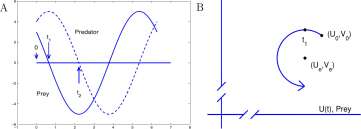
Figure 7.11: A. Conventional and B. phase graphs of predator prey functions. For scale, the distance from (U e , V e ) to (U 0 , V 0 ) is 5.
b. What are w'(0) and u'(0)?
c. On your replica of Figure 7.11 A, draw tangents to the graphs of u and v at u(0) and v(0).
d. On your replica of Figure 7.11B draw a line from (C/q, Vq) to (Uq + u'(0), Vq + v'(0)). Note that the distance from (U e , V e ) to (U 0 , V 0 ) is 5.
e. In Figure 7.11 A, at the time t = 0 the prey curve has negative slope and the predator curve has positive slope. The graph in Figure 7.11B moves from (Uq,Vq) to the left (prey is decreasing) and upward (predator is increasing).
1. Discuss the dynamics of the predator and prey populations at time t\.
2. Discuss the dynamics of the predator and prey populations at time t<x marked on Figure 7.11A and mark the corresponding point on Figure 7.11B.
f. Show that
(u(t)) 2 + (v(t)) 2 = ul + vl What is the significance of this equation?
Exercise 7.5.6 J. D. Murray Mathematical Biology, Springer, New York, 1993, p 66 observes an exception to the phase graph for the Lynx-Hare during years 1874-1904. The data are shown in Figure 7.12 along with a table of part of the data.
a. Read data points in Figure 7.12 for the years 1887 and 1888.
b. Use the data in Table 7.2 and your two data points to make a phase plot for the years 1875 – 1888.
c. Discuss the peculiarity of this predator-prey phase plot.
Murray notes that the 1875 – 1887 data seems to show that the ‘hares are eating the lynx’, and cites some explanations that have been offered, including a possible hare disease that could kill the
CHAPTER 7. DERIVATIVES OF THE TRIGONOMETRIC FUNCTIONS
331
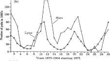
Figure 7.12: Snowshoe Hare and Lynx data for the years 1874-1904.
Table 7.2: Lynx-Hare data read Figures 3 (hare) and 16 (lynx) of D. A. MacLulich, Fluctuations in the number of varying hare, University of Toronto Studies, Biological Sciences, No. 43, 1937.
Hare Lynx Data Read From the Graph
lynx (no such disease is known) and variation in trapping practice in years of low population density.
Exercise 7.5.7 For the algebraically robust. For Equations 7.34 and 7.35,
u(t) = —Vq sm(Vab t) + u 0 cos(v / a6 t) v(t) = v 0 cos(y / a6 t) + uq\\ — sin(y / a6 t) V o V a
show that
^(^)) 2 + ^(,(t)) 2 = ^(. 0 ) 2 + ^(,o) 2 .
a
What is the significance of this equation?
Exercise 7.5.8 Suppose the prey population may be affected by over crowding even with low predator presence.
Mathematical Model 7.5.2 For small deviations, u{t) and v(t), from equilibrium, we assume that
1. The prey population decreases, U'(t) is negative, when there is excess prey population u(t) and when there is excess predator population, v(t).
2. The predator population increase, V'(t), is proportional to the excess prey population, u(t).
CHAPTER 7. DERIVATIVES OF THE TRIGONOMETRIC FUNCTIONS
332
Step 1 can be interpreted at least two ways:
A. —U'(t) could be proportional to the product of u(t) and v(t), or
B. —U'(t) could be proportional to the sum of av(t) + cu(t) where a and c are numbers. Both interpretations are relevant. Here we choose interpretation B. Step 2 is the same as for
Model 7.37 and write
-U'(t) = av{t) + cu(t)
V'(t) = bu(t) Again U'{t) = u'(t) and V'(t) = v'(t), so that
u'(t) = —av(t) — cu(t)
(7.37)
v ‘{t) = bu(t)
a. Use Equations 7.37 to show that
v”(t) + cv'(t) + abv(t) = 0 (7.38)
Hint: Compute
[v'(t)]’ = [bu(t)]’, use u'{t) =-av{t) – cu{t) and bu{t)=v'{t)
b. Equation 7.38 may be compared with Equation 7.28 for damped harmonic motion (harmonic motion with resistance). For a = 2.02, b = 0.5, and c = 0.2 the equation becomes
v”(t) + 0.2 v'(t) + 1.01 v(t) = 0 (7.39)
Show that
v (t) =e-^ w smt
is a solution to this equation.
c. Show that if v(t) = e _ */ 10 sint then
u(t) = 2e~ t/w cost – 0.2e^ /10 sint
d. Show that
u 2 + OAuv + 4.04 v 2 = 4e” t/5
e. Plot a graph of u(t) vs v(t). It is of interest that u 2 + 0.4 uv + 4.04 v 2 = 4 is an ellipse in the u-v plane.
7.6 Periodic systems.
Many biological and physical systems exhibit periodic variation governed by feed back of information from the state of the system to the driving forces of the system. An excess of predators (state of the system) drives down (driving force) the prey population. An elongation of a spring (state of the system) causes (driving force) the suspended mass to move up toward the equilibrium position.
Examples of periodically varying feed back systems are presented. Exercises are distributed through the three subsections.
CHAPTER 7. DERIVATIVES OF THE TRIGONOMETRIC FUNCTIONS
333
Explore 7.6.1 Chamelons are a group of lizards that change their color to match the color of their environment. What is the color of a chamelon placed on a mirror? ■
7.6.1 Control switches.
Some street lights and household night lights have photosensitive switches that turn the lights on at sunset and turn them off at sunrise. In Figure 7.6.1 is a household night light with a photosensitive switch and a mirror. The mirror can be adjusted so that the light from the bulb is reflected back to the photosensitive switch. What will be the behavior of the switch at night? With sunlight shining on it?
Explore 7.6.2 You will find it interesting to perform an experiment. In a dark room, hold a mirror about 3 inches from a night light so that it reflects light from a night light back to the photosensitive switch. Move the mirror about 8 inches from the night light and note the change in the activity of the night light. ■
We propose the following mathematical model for the system.
Mathematical Model 7.6.1 Night lights. I There is a voltage in the photosensitive switch that increases at a rate proportional to the intensity of light striking the switch and the intensity of the light leaving the bulb decreases at a rate proportional to the voltage.
The intensity of the reflected light that strikes the switch is proportional to the intensity of the light leaving the bulb and inversely proportional to the square of the distance from the bulb to the mirror.
Exercise 7.6.1 a. The first paragraph should remind you of a predator prey system. Assuming so, is the voltage the predator or the prey?
b. Write equations for the mathematical Model 7.6.1.
Figure for Exercise 7.6.1 A night light with a mirror that can be positioned to reflect light back
to the photosensitive switch.
CHAPTER 7. DERIVATIVES OF THE TRIGONOMETRIC FUNCTIONS
334
Exercise 7.6.2 We propose a second mathematical model for night lights.
Mathematical Model 7.6.2 Night lights. II There is a voltage in the photosensitive switch that increases at a rate proportional to the intensity of light striking the switch and dissipates at a constant rate when no light strikes the switch. The light is either on or off; it turns on when the voltage falls below a certain threshold and turns off when the voltage exceeds another threshold.
The intensity of the reflected light that strikes the switch is proportional to the intensity of the light leaving the bulb and inversely proportional to the square of twice the distance from the bulb to the mirror.
Let v(t) be the voltage in the photosensitive switch at time t and i(t) be the illumination striking the photosensitive switch at time t.
a. Write an equation descriptive of
There is a voltage in the photosensitive switch that increases at a rate proportional to the intensity of light striking the switch and dissipates at a constant rate when no light strikes the switch.
b. Because the light is either on or off, it is easiest to treat the mathematical model 7.6.2 Night Light II as a discrete system. Choose an increment time 5 > 0 and for k — 0,1, 2, • • • N, let
Vk = v(k x 5) and i k = i(k x 5),
and assume that
in x\ ■ Vk + 1 ~ Vk v (k x d) = .
o
Write a discrete analog of your previous equation
c. Let v on < v Q ff be threshold values and sw(v) be a ‘switch’ function defined by
1 for v(t) < v on
sw(v(t)) = (1 + sign(v'(t)))/2 for v on < v(t) < v off 0 for v 0 fj < v(t)
Figure 7.6.2 illustrates the solutions to the equation
v 0 = 1.25 to = 0
v k+l = v k + (2 x i k – 1) x 5 (7.40)
i fc+ i = sw(v k ), where v on = 1.5 and v Q ff = 2.5, and N = 230.
If you have adequate computing, replicate Figure 7.6.2. Else, compute (vi,ii), (^2,^2), (^3,23), (v 4 ,u), and (v 5 ,i 5 ).
Figure for Exercise 7.6.2 Solutions to Equations 7.40. Light intensity is the solid curve and
voltage is the dashed curve.
CHAPTER 7. DERIVATIVES OF THE TRIGONOMETRIC FUNCTIONS
335
3 2.5
1.5
c
.0
(3
0.5 0
0 50 100 150 200 250
Time
Exercise 7.6.3 Thermostats control the furnaces on houses. They turn the furnace on when the temperature falls below a temperature set by the home owner and turn the furnace off when the temperature exceeds a temperature set by the home owner.
Figure 7.13: Inside view of a Honeywell thermostat. The coil is expanded and the mercury is at the right end of the tube and does not connect the wires at the opposite end.
The control system of a thermostat is shown in Figure 7.13. There is a bi-metalic coil that expands or contracts according to the temperature of the coil. There is a small glass tube containing a dollop of mercury at the top of the coil that tilts as the coil expands or contracts. Three wires are at one end of the tube. When the temperature is “low” the tube tilts so that the mercury completes the connection between the two wires. When the temperature is “high” the tube tilts so that the mercury is at the opposite end of the tube from the wires and the connection is broken. As the temperature moves between the “low” and “high” temperatures the mercury slowly moves towards the center of the tube until a threshold angle is reached and it flows to the opposite end of the tube and either opens or closes the connection between the two wires.
a. Write a mathematical model descriptive of temperature inside a house when the furnace is
CHAPTER 7. DERIVATIVES OF THE TRIGONOMETRIC FUNCTIONS
336
not running and the outside temperature is below the temperature inside the house. You may wish to review Exercises 1.11.5 and 5.5.23 and 7.6.2.
b. Write equations that describe your mathematical model.
c. Draw a graph descriptive of the temperature inside a house in northern Minnesota for one day in January.
d. Draw a graph descriptive of the temperature inside a house in Virginia for one day in January.
7.6.2 Earthquakes.
The San Andreas fault in California is an 800 mile zone of contact between two tectonic plates, with the continental crust on the east and the oceanic crust on the west. As the oceanic crust moves north and rubs against the continental crust, at some points along the fault faces of the crust lock together and the earth bends — until a threshold distortion is surpassed. Then the faces of the crusts abruptly slide past one another sending shock waves out across the earth, and the crusts returns to a more relaxed condition. The maximum slippage recorded between two crusts is a 21 foot displacement of a road during the 1906 earthquake in the San Francisco region.
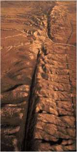
Figure 7.14: San Andreas Fault. Photograph from Wallace, Robert E., ed., 1990, The San Andreas fault system, California: U.S. Geological Survey Professional Paper 1515, 283 p. [http://pubs.usgs.gov/pp/1988/1434/].
CHAPTER 7. DERIVATIVES OF THE TRIGONOMETRIC FUNCTIONS
337
A simple model of this system was described by Steven Gao of Kansas State University. Consider a body of mass m on a horizontal platform, a spring with one end attached to the body and the other end moving along the platform at a rate v. There are two frictions associated with the body, the starting friction, F start , and the sliding friction, F s ud e ,
Fslide *^ Fstart-
If the body is not moving relative to the platform, F sta rt is the force required to initiate movement. If the body is in motion along the platform, F s ud e is the force required to continue motion.
The spring has a spring constant k; an elongation of length E in the spring causes a force of magnitude k x E on the body. Let L be the length of the spring when there is no tension on the spring.
A
y(0) = L
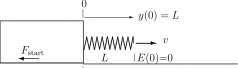
x(0) = 0 0
B
^start = k Vt]_
y(ti)
WAA/VWVWWW— 1
L \E(t 1 ) = vti
x(h) = o
c

/wwvwwwv
-y(t)
L \E(t)
x(t)
Figure 7.15: A. Initial condition of a block with spring pull and starting friction. B. The block will first move at time t\ when the force of the spring elongation, kvti, exactly matches the starting friction, Fstart- C. Motion of a block with spring pull and sliding friction.
In this model, the horizontal platform is the continental crust and the body and spring are the oceanic crust.
Mark a point on the platform as the zero point, let x(t) be the distance from zero to the forward face of the body, and let y(t) be the distance from zero to the forward end of the spring. Let E(t) be the extension of the spring.
Assume the initial conditions:
x(0) = 0, y(0) = L, so that E(0) = 0
Exercise 7.6.4 1. What is y'(t) for all t?
CHAPTER 7. DERIVATIVES OF THE TRIGONOMETRIC FUNCTIONS
338
2. Write a formula for y(t).
3. The force of the spring on the body will be k x E(t) = k (y(t) — L — x(t)). What is the force at time t — 0?
4. At what time, t 1: will the body first move (will the force on the body = F start )7
During the first motion of the body, the net force, F, on the body will be
F = k (y(t) — L — x(t)) — F sUde = k (L + vt – L – x(t)) – F slide
= k (Vt- X(t)) – F s iide
Newton’s second law of motion gives
F = m a = m x” ,
so that
mx” = k (vt – x(t)) – FsUde
or
x” + u J 2 x=-vtF ^ u? = – (7.41)
mm m
Let t\ be the time at which the first motion starts. Then
x(t x ) = 0 (7.42) ar'(ti) = 0 (7.43)
Reader Beware: Incoming Lightning Bolt! In Chapter 17, Second order and systems of two first order differential equations, you will learn how to find the function, x(t), that satisfies equations 7.41, 7.42, and 7.43:
/.\ F s i ar i -\- F s nde / /. . \\ X[t) = : COS (OJ [t — t\))
k
–80^-^)) + ^-% (7.44) uj k
Exercise 7.6.5 Show that the function, x(t) defined in Equation 7.44 satisfies equation 7.42, 7.43, and 7.41.
Exercise 7.6.6 Equation 7.44 is valid until x'(t) next equals to zero. Use the parameters
Fstart = 5, FsUde = 4, k = 1, v = 0.1, and m = 1
and draw the graph of x. An elongation of E = F s tart/k = 5 initiates motion at time
t\ = i^t^t /kv = 50, and uj 2 = k/m = 1 with these parameters. Find the time and value of x at
which x’ — 0.
Using the parameters of the previous exercise, the body moved 2.33 units in a time of 3.33 units; the velocity of the forward end of the spring is 0.1 so the forward end moved 0.33 units during the motion. At the time the body stopped moving, the elongation of the spring was 5 – 2.33
CHAPTER 7. DERIVATIVES OF THE TRIGONOMETRIC FUNCTIONS
339
B
Q) 4
01
CC
a a
ui 3
0 10 20 30 40 50 60 70 80 90 100 110
Time – t
Figure 7.16: A. Graph of the first slippage, x(t) } for Equation 7.44 and the parameter values of Exercise 7.6.6. B. Graph of three slippage events with quiescence between events.
Table 7.3: Significant earthquakes in the Los Angeles, CA area 1920 – 1994, http://pasadena. wr.usgs.gov/info/index.html
+ 0.33 = 3. After 20 more time units, the elongation will again reach 5 and the motion of the body will be repeated. A graph of the motion of the body is shown in Figure 7.16
The model we describe exhibits periodic ‘relief of the tension in the spring. Do earth quakes exhibit periodicity in their recurrence? If so it would greatly simplify the prediction of earth quakes! The dates of significant earth quakes and their magnitudes (4.8 – 6.7) that have occurred in the Los Angeles area fault since 1920 are shown in Table 7.3. You may search the table for periodicity. As emphasized by Dr. Gao, the fault is a complex system; many small earthquakes occur every month; relief in on section may increase strain at other points. His model does, however, suggest the nature of the mechanics of an earth quake. The U.S. Geological Survey web site, http://pubs.usgs.gov/gip/earthq3/, contains very interesting discussion of earthquakes.
7.6.3 The circadian clock.
Exciting current studies in molecular biology and genetics are illuminating the molecular and neural systems that control the daily rhythm of our lives, wakes us up in the morning, puts us to sleep at night, and causes ‘jet lag’ when we travel to different time zones or even without travel when daylight savings time is initiated in the Spring. The molecular clocks that control circadian rhythms have been identified in fruit flies, mammals, Neurospora (fungus), Arabidopsis (plant), and cyanobacteria. They are markedly similar and It appears that there has been multiple evolution of
A
2.5 –
Q.
0.5 –
0
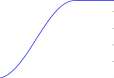
48 49 50 51 52 53 54
CHAPTER 7. DERIVATIVES OF THE TRIGONOMETRIC FUNCTIONS
340
the same basic mechanism. The Neurospora mechanism is described here from a review, J. C. Dunlap, Ann. Rev. Genet. 30 (1996), 579.
In Neurospora, there is a gene, frq (frequency), that is transcribed into a mRNA also called frq that codes for a protein, denoted FRQ. FRQ stimulates metabolic activities associated with daylight. A high level of FRQ also acts to shut off transcription of the gene frq so that the concentration of mRNA frq decreases. There is a potentially oscillating system: frq increases and causes an increase in FRQ that causes a decrease in frq so that FRQ decreases (is no longer transcribed from frq and is naturally degraded as are most proteins). However, there is resistance in the system and periodic stimulus from daylight is necessary to keep the system active and to entrain it to the daily 24 hour rhythm.
Circadian time (CT) begins with 0 at dawn, 6 is noon, 12 is dusk, 18 is midnight, and 24 = 0 is dawn. The Neurospora circadian cycle begins at midnight, CT 18, at which time both frq and FRQ are at low levels, but transcription of frq begins, say at a fixed rate. After a 3 hour time lag translation of frq to create FRQ begins. At dawn, CT 0, there is a marked increase in transcription of frq and an almost immediate increase of translation to FRQ. A high level of FRQ inhibits the transcription of frq and frq levels peak during CT 2-6 and declines steadily until CT 18. FRQ levels peak during CT 6-10 and also decline until CT 18 (the protein FRQ is constantly degraded and with decreasing levels of frq the turnover is more rapid than production).
Exercise 7.6.7 a. Draw a graph representative of the concentration of the mRNA frq as a function of time (use CT).
b. Draw a graph representative of the concentration of the protein FRQ as a function of time (use CT).
c. Draw a phase diagram with concentration of frq on the horizontal axis and concentration of FRQ on the vertical axis covering one 24 hour period.
Chapter 8
Applications of Derivatives.
Where are we going?
The derivative is a powerful tool for analysis of curves, selection of optimal parameter values, and measuring the influence of one variable on another. If you are a doctor in the midst of a flu epidemic, you know that the number of newly infected people is increasing every day. What is important to you today is whether the rate at which newly infected people appear is increasing suggesting a future similar to A or is slowing down as in B. B is better.
If the graphs represent the daily weight of an infant, however, B. could be a signal of inadequate nutrition or disease. A is better

Today
Time days
8.1 Some geometry of the derivative
It is often important to know whether a population, atmospheric CO2 concentration, average temperature, white blood count, number of flu cases, etc. is increasing or decreasing with time or location, and whether the rate of increase is itself increasing or decreasing.
The relation between positive, negative, and zero slopes and increasing, nondecreasing, nonincreasing, decreasing, highest points and lowest points is examined. The graph in Figure 8.1 illustrates three of these concepts. The graph has positive slope at every point, and is increasing. The slopes increase between points A and B, and the tangents lie below the graph. The slopes decrease between points C and D, and the tangents lie above the graph.
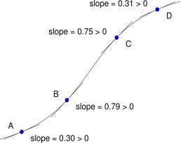
Figure 8.1: Graph of an increasing function. The slope is positive at every point. Between points A and B the slopes increase from 0.3 to 0.79 and the tangents lie below the curve. Between point C and D the slopes decrease from 0.75 to 0.31 and the tangents lie above the curve.
In Definition 3.1.3, the derivative P'(a) of a function P(t) at a number a is the slope of the tangent to the the graph of P at the point (a, P(a)).
The next definition of increasing function should agree with your intuitive notions that a population is growing, or that a chemical is accumulating, or a that temperature is increasing.
Definition 8.1.1 A function P, is said to be increasing if for any two numbers, a and b in the domain of P,
if a <b, then P{a) < P(b).
Explore 8.1.1 Do this.
1. Only one of the graphs shown in Figure 8.1.1 is the graph of an increasing function. Which one?
2. For the function that is not increasing, explain why it fails to satisfy Definition 8.1.1.
3. Does every tangent to the graph of the increasing functions have positive slope?
Explore Figure 8.1.1 Graphs of an increasing function and a function that is not increasing.
CHAPTER 8. APPLICATIONS OF DERIVATIVES
343
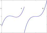
It may seem intuitive that if a population is growing then the growth rate is always positive. This is not true – as you may have found out from the preceding Explore 8.1.1 and is shown in the next example.
Example 8.1.1 A graph of the cubic function, P(t) = t 3 is shown in Figure 8.1.1.1 (and in Explore Figure 8.1.1), together with the tangent to the graph at the point (0,0). P(t) = t 3 is an increasing function: If a < b then a 3 < b 3 .
However, the tangent to the graph of P at (0,0) is horizontal. P'(0) = 3 t 2 \ t=0 = 3 0 2 = 0. So that P’ is not everywhere positive.
Figure for Example 8.1.1.1 The graph of y = t 3 and its tangent at (0,0).
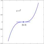
-1.5 -1 -0.5 0 0.5 1 1.5
The previous example is a bit of a nuisance. We would like increasing function and positive slope to be equivalent, and they are not. The fall back position is to define non-decreasing functions which will be found to be equivalent to non-negative slopes.
Definition 8.1.2 A function P, is said to be non-decreasing if for any two numbers a and b in the domain of P,
if a < 6, then P(a) < P{b).
Note: Compare
If a < b then P{°) < P(b)- Increasing
and
If a < b then P( a ) < Pip)- Non-decreasing
CHAPTER 8. APPLICATIONS OF DERIVATIVES
344
Every increasing function is also non-decreasing, but, for example, a constant function, P(t) = C, is non-decreasing but is not an increasing function.
Explore 8.1.2 Suppose P is a non-decreasing function.
a. Argue that every difference quotient, P( ^lf — , is greater than or equal to zero. (Consider two cases: a < b and b < a.)
b. Suppose a is a number for which P'{a) exists. Argue that P'(a) is not a negative number.■
Thus if P is a non-decreasing function, then P'(t) > 0 for all t (P’ is nonnegative). This result is often used in reverse:
If P'(t) > 0 for all t then P is non-decreasing.
That is a true statement and is Theorem 12.2.1 of Section 12.2. We use it in this chapter, but we have not yet shown it to be true.
The two results may be written as a theorem to be proved in Section 12.2.
Theorem 8.1.1 Suppose P is a function defined on an interval [a, b]. Then P is nondecreasing on [a, b] if and only if P'(t) > 0 for all t in [a, b].
Explore 8.1.3 Write definitions of decreasing function and of non-increasing function and state a theorem about nonincreasing functions analogous to Theorem 8.1.1. ■
We also state a related theorem to be proved in Section 12.2:
Theorem 8.1.2 Suppose P is a continuous function defined on an interval [a, b]. If P'(t) > 0 for a < t < b then P is increasing on [a, b].
That the converse of this theorem is not a theorem follows from the example of P(t) = t 3 , [a,b} = [-1,1].
Example 8.1.2 The natural logarithm, In, is an increasing function.
By the previous theorem, In is increasing if In’ is positive. In a; is only defined for x > 0, and
[In a]’ = – > 0 for x > 0
Explore 8.1.4 Is it true that In is a nondecreasing function?
CHAPTER 8. APPLICATIONS OF DERIVATIVES
345
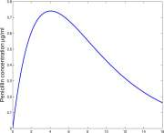
Time — hours
Figure 8.2: The graph of C(t) = 5e 0,24 — 5e 0 34 showing a period of increasing blood penicillin concentration followed by a period of decreasing blood penicillin concentration.
Example 8.1.3 Following ingestion of a penicillin pill, penicillin is absorbed from the intestine into the blood stream, the concentration, C, of penicillin in the blood is approximated by the function
C(t) = 5e~ a2i – 5e-° M ^
ml
where t is time measured in hours (Figure 8.2).
Problem: During what time interval is the concentration of penicillin in the blood increasing? What is the maximum concentration of penicillin? Solution: Compute
C'{t) = [5ea2t – 5e-°’ 3 ‘~’
= 5e-°’ 2 * (-0.2) – 5ea3t (-0.3)
= 5 e-°3t (-0.2e aii + 0.3)
Because 5 > 0 and e _0,3t > 0 for all t, C'(t) is positive if —0.2e 01t + 0.3 is positive. The following inequalities are equivalent:
-0.2e !
O.lt
0.3 > 0
We can conclude that C'(t) is positive if 0 < t < 10 In 1.5 = 4.05. Thus serum penicillin is increasing for about four hours after ingestion of the penicillin pill into the intestinal track. ■
CHAPTER 8. APPLICATIONS OF DERIVATIVES
346
You were asked in Explore 8.1.3 to define decreasing and nonincreasing.
As in Explore 8.1.2, you can show that if P is nonincreasing, then P'(t) < 0. By considering Q(t) = —P(t), it follows from Theorem 8.1.1 that if P'(t) < 0 then P is nonincreasing, and from Theorem 8.1.2 that if P'(t) < 0 for a < t < b then P is decreasing on [a, b].
From the preceding example of blood penicillin concentration, with C'(t) = 5 e-°3t (-0.2e ai * + 0.3) we observe that
5 > 0 e-° M > 0 for all t and – 0.2e 01t + 0.3 < 0 for 10 In 1.5 < t
and we conclude that penicillin concentration is decreasing for t > 10 In 1.5 = 4.05 hours.
Because the penicillin concentration is increasing during 0 to 10 In 1.5 hours and decreasing afterward, the maximum concentration must occur at 10 In 1.5 hours. That maximum concentration is C(101nl.5) and
C(l01nl.5) = 5e -0.2xl01nl.5_ 5e -0.3xl01nl.5 = 5e -21nl.5_ 5e -31nl.5
= 5(e lnL5 )~ 2 -5(e lnL5 )~ 3
\ l r, “A 3 = °74074 -Hence, the maximum concentration is approximately 0.74 /ig/ml.
Explore 8.1.5 Draw the tangent to the graph in Figure 8.2 at the point(4.05, 0.74). ■
8.1.1 Convex up, concave down, and inflection points.
Now we examine when P’ is increasing (signaled by P” > 0). In such regions, the graph of P is convex up or simply convex. Similarly, when P” < 0, P’ is decreasing and the graph of P is concave down or simply concave. Information provided by the second derivative is illustrated by the graph of P(x) = x(x – 2) (x – 4) = x 3 – 7x 2 + lOx in Figure 8.3.
p{x) = x 3 – 7x 2 + lOx, P'(x) = 3x 2 – Ux + 10 P”( x ) = 6x-U = 6(x-7/3)
In Figure 8.3, the slope of P decreases on the interval [A, a}. The slope of P increases on the interval [b,B].
If x < 7/3, P”(x) < 0, and P'(x) is decreasing and P(x) is concave down.
If x < 7/3, P”(x) > 0, and P'(x) is increasing and P(x) is convex up.
The tangents to the graph at A and a lie above the graph except at the points of tangency, consistent with P being concave down onx< 7/3. The tangents to the graph at b and B lie below the graph except at the points of tangency, consistent with P being convex up on 7/3 < x. The point at (7/3,19/3) is an inflection point. P”(7/3) = 0 and the tangent at (7/3,19/3) crosses the graph.
CHAPTER 8. APPLICATIONS OF DERIVATIVES
347
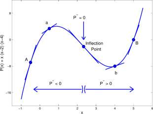
Figure 8.3: Graphs of P{x) = x(x — 2)(x — 4). a. The slope is decreasing on (—oo, 7/3); the tangents lie above the graph except for the points of tangency and the graph is concave down. b. (7/3, 19/3) is an inflection point; the tangent crosses the graph at that point. The slope is increasing on (7/3, — oo); the tangents lie below the graph except for the points of tangency and the graph is convex up.
8.1.2 The arithmetic mean is greater than or equal to the geometric mean.
We prove here Theorem 5.2.2 which was stated without proof in Subsection 5.2.1 in which the number e was shown to be lim (1 + h) l ‘ h .
h— >0
Theorem 5.2.2. If oi, a 2 , • • •, a n is a sequence of n positive numbers then
ai + a 2 + ■ ■ •
n
> yaia 2 ■■■a n (8.1)
with equality only when a\ = a 2 = ■ ■ ■ = a n .
In the proof we use the facts that for any integer n > 1
1 + (n – 1) ( n \/*) = nVi for t=l (8.2) l + (n-l)( n Vt) > nZft for t>l (8.3)
Proof of Equations 8.2 and 8.3. Suppose n > 1 is an integer and
F(t) = 1 + (n – 1) ( n ~Vt) – ny/i = 1 + (n – 1) – nt^
Then -F(l) = 1 + (n — 1) x 1 — nx 1 = 0 and Equation 8.2 is satisfied. Next F'(t) is computed as
CHAPTER 8. APPLICATIONS OF DERIVATIVES
348
0 + (n – 1
i i -i i i
i 1″1 -n-W
n — 1 n
_ n-1 _ n-1
t n-1 _ £ n
= i «-i 1 -1
For t > 1 both factors are greater than zero and -F'(i) > 0 for t > 1. It follows from Theorem 8.1.2 that F is increasing for t > 1. Because F(l) = 0 and F is increasing for t > 1, for t > 1
F(t) > 0
l + (n- 1) ” -Vi-riVi > 0
l + (n-l)”v^ > nv^ Equation 8.3 is satisfied, h End of proof of Equations 8.2 and 8.3.
Proof of Theorem 5.2.2. We proceed by induction. First we prove that if a x and a 2 are two positive numbers then (ai + 02)/2 > 0,10,2-
( ai -a 2 ) 2 > 0
a 2 — 2a x a 2 + a 2 > 0
a 2 + 2aia 2 + a 2 > 4aia 2 (ai + a 2 ) 2
1 > aia 2
ai + a 2
—2— > vaia 2
Furthermore, (ai — a 2 ) 2 = 0 only when a,i = a 2 and equality holds in each expression of the previous array only when a x = a 2 . The statement in Theorem 5.2.2 is valid with n = 2.
Now suppose n is an integer, n > 3, and Equation 8.1 is valid for sequences of length n — 1 and ai, a 2 , ■ • ■ a n is a sequence of positive numbers of length n. We assume without loss of generality that a n is the smallest number in ai, a 2 , • • • a n , and consider the sequence 6^ — Q,k/o, n , k — 1,ti. Then 6 fc > 1 and b n = 1. Consequently,
£ = … bn-xbn = b ± b 2 ■ ■ ■ 6„_i > 1
with equality only for 61 = 6 2 = • • • = b n ~i = 1. Observe that b± = b 2 = ■ ■ ■ = 6 n -i = 1 only if ai = a 2 = ■ • • = a n .
From Equations 8.2 and 8.3 we know that 1 + (n – 1) “”v^ >ny/i for t > 1 with equality only for t = 1. Therefore
CHAPTER 8. APPLICATIONS OF DERIVATIVES
349
By the induction hypothesis
bi + b 2 + ■ ■ ■ 6 n _x > (ra – 1) ( “-^6162 •••6n-i) ,
so that
1 + 61 + 62 + • • • &„_i > 1 + (n – 1) ( n -^6i6 2 —6 n _i) ,
Multiply all all terms by a n and we get
fl„ + ai + a 2 H a n _i > n ^/aia 2 • • • a n
or
ai + a 2 H a n
n
Equality holds in the previous five expressions only if b± — b 2 — ■ ■ • — 6 n _i = 1, in which case a 1 = 0,2 — • • • — In-End of proof.
Exercises for Section8.1, Some geometry of the derivative.
Exercise 8.1.1 Argue that e x is an increasing function.
Exercise 8.1.2 Argue that sin a; is an increasing function on 0 < x < n/2.
Exercise 8.1.3 Suppose penicillin concentration is given by C(t) = 8e~ a2t — 8e~ 0At /igm/ml t hours after ingestion of a penicillin pill. For what time period is the concentration increasing? What is the maximum penicillin concentration?
Exercise 8.1.4 Suppose penicillin concentration is given by C(t) = 0.4te -0 ‘ 5 ‘ /igm/ml t hours after ingestion of a penicillin pill. For what time period is the concentration decreasing? What is the maximum penicillin concentration?
Exercise 8.1.5 Identify the intervals, if any, on which f(x) is increasing and intervals, if any, on which /’ is increasing.
CHAPTER 8. APPLICATIONS OF DERIVATIVES
350
Exercise 8.1.6 We show in Chapter 9 that if n is an integer then
/ i \ n(n + l)
l + 2 + — -(n-l)+n = —-.
Use this and Theorem 5.2.2 to show that if n is an integer

where n\ — 1 • 2 • 3 • • • (n — 1) • n.
Exercise 8.1.7 Trout, Moose, and Bear lakes are connected into a chain by a stream that runs into Trout Lake, out of Trout Lake into Moose Lake, out of Moose Lake and into Bear Lake and out of Bear Lake. The volumes of all of the three lakes are the same, and stream flow is constant into and out of all lakes. A load of waste is dumped into Trout Lake. With t measured in days and concentration measured in mg/1, the concentration of wastes in the three lakes is projected to be
Trout Lake: C T (t) = O.Ole” 0 05 * Moose Lake: C M (f) = 0.005te-°05t
Bear Lake: C B {t) = 0.000025^ e -°05 ‘ For each lake, find the time interval, it any, on which the concentration in the lake is increasing.
8.2 Some Traditional Max-Min Problems.
We present a few of the large number of interesting optimization problems that are part of the culture of calculus. The basis for solving these problems is the following definition and theorem.
CHAPTER 8. APPLICATIONS OF DERIVATIVES
351
In Figure 8.4, the point B is a maximum for the graph and an interior maximum. The points A and C are local minima for the graph; A is an endpoint local minimum and C is an interior local minimum. The point D is an interior local maximum and E is an endpoint minimum.
B
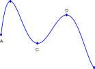
E
Figure 8.4: Maxima and minima. A is an endpoint local minimum, B is an interior maximum, C is an interior local minimum, D is an interior local maximum, E is an endpoint minimum.
If (c, /(c)) is a maximum for / then we may say that / attains its maximum value at c, or the maximum value of / occurs at c, or that the maximum value of / is /(c). Thus, the sine function attains its maximum value at | and the maximum value of the sine function is 1. Also the sine function attains its minimum value at ^ and the minimum value of the sine function is -1. The function f(t) = t 3 does not have a maximum value and does not have a minimum value. The word, ‘value’, is often omitted in these statements, and we may say, for example, that 1 is the maximum of the sine function and f(t) = t 3 has neither a maximum nor a minimum. Similar language is used with local and interior local maxima and minima.
Theorem 8.2.1 If (c,/(c)) is an interior local maximum for a function, /, and
if /'(c) exists, then f'(c) = 0.
(Equivalently, if the graph of / has a tangent at an interior local maximum (c, /(c)), then that tangent is horizontal.)
Proof. Suppose (c, /(c)) is an interior local maximum for /, and (p, q) is an interval in D containing c for which f(x) < /(c) for all x in (p, q). We wish to show that /'(c) = 0. See Figure 8.5. Suppose p < b < c. Then b — c < 0, and because c is a local maximum
f(b)<f(c) and /(6)-/(c)<0 and M Z ^ > 0
It follows that
/<-(e) = lim W>-W > 0. J y ‘ b^c- b-c
CHAPTER 8. APPLICATIONS OF DERIVATIVES
352
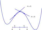
Figure 8.5: A local maximum and left and right secants.
Similar analysis shows that
c) = lim
fib) – /(c)
< 0.
b^c+
b-C
If /'(c) exists, /'(c) = f’-(c) and /'(c) = f+(c). Therefore, /'(c) = 0. End of Proof.
2. /'(c) does not exist, or
3. c is either a or b.
The points c satisfying either 1, 2, or 3 are called the Critical Points for /
on [a, b].
In the examples considered in this book, there are usually only a few (no more than five, say) critical points. Then finding the maximum and minimum values only involves selecting from among at most five values of /.
Example 8.2.1 Suppose you are going to make a rectangular box with open top from a 3 meter by 4 meter sheet of tin. One procedure for doing so would be to cut squares of side x from each corner as shown in Figure 8.6A, and to fold the ‘tabs’ up. Four pieces of area x 2 would be discarded. What value of x will maximize the volume of the box you construct in this way? What will be the volume of the box of largest volume?
After the corners are cut, the ‘core’ of the tin that will make the bottom of the box will be of length 4 — 2x and width 3 — 2x. The height of the box will be x and the volume of the box formed will be
Summary: Critical Points.
If c is a local maximum or local minimum for a function, /, defined on an interval [a, b] then
1
/'(c) = 0, or
V = (A – 2x)(3 – 2x)x

CHAPTER 8. APPLICATIONS OF DERIVATIVES
353