part0006

pW(l) = f(k)(!)

p(x) = 7T 0 + 7Ti (X ~ 1) + 7T 2 (x – l) 2 + 7T 3 (x – l) 3 p(l) = 7T 0 7T 0 = 0

p'(x) = 7r 1 + 2 7r 2 (:r-l) + 3 7r 3 (:r-l) 2 = tti ^ = 1

p( 2 )(:r) = 2 7r 2 + 3-27r 3 (x-l) = 2tt 2 tt 2 = -|

p( 3 )(x) = 3-2vr 3 p( 3 )(l) = 3-2tt 3 tt 3 = |

As for the quadratic, 7r 0 = 0, tt± — 1, and 7r 2 = — |. The only new term is 7r 3 (x — 3) 3 = | (rr — 3) 3 and the cubic is

p(x)=0 + l-(x-l)1 2 (x-iy+ 1 3 (x-l) 3

General form of the coefficients. There is a general pattern to the coefficients for an approximating polynomial with anchor point a when the polynomial is expanded in powers of (x — a).

We treat the case of a third degree polynomial to illustrate the pattern.

Assume we are given a function, /, which has first, second, and third continuous derivatives and a number, a, in its domain.

Then the third degree polynomial that matches / at a is

f (2) (a) f (3) (a) p(x) = f(a) + f'(a)(x -a) + L ^ 1 (x – af + J —^ J -{x – af

The lower and higher degree polynomials that match / at a have a similar form.

We show the validity for the third degree polynomial. Let

p(x) = 7r 0 + ni (x – a) + 7r 2 (x – a) 2 + ir 3 (x – a) 3

and observe that

p(x) = 7T 0 + TTi (x – a) + 7T 2 (x – a) 2 + 7T 3 (x – of p(d) = 7T 0

p'{x) = iii + 2 7T 2 (x — a) + 3 7r 3 (x — a) 2 P'( a ) — n i

p {2 \x) = 27r 2 + 3-27r 3 (a:-a) p^ 2 \a) = 2! tt 2

CHAPTER 12. THE MEAN VALUE THEOREM; TAYLOR POLYNOMIALS

535

Now the requirement that p^ k \a) = f^ k \a) leads to

p(a) = f(a) p'(a) = f'(a)

P p) (fl) = / (2) («)

p^(a)

/(3) ((

7T 0

2! vr 2

3! 7T 3

/(«) /»

/ {2) («) / {3) («)

7T 0

/(«) /'(a)

vr – ^ 7T 2 – 2!

The general form for the cubic approximating polynomial with anchor point, a, is p(x) = f(a) + f(a) ( x -a) + ^(x- a) 2 + (x – a) 3

2!

Lower and higher order polynomials have similar forms.

3!

Example 12.6.1 Suppose you are monitoring a rare avian population and you have the data shown. What is your best estimate for the number of adults on January 1, 2003?

Let t measure years after the year 2000, so that t — 0, t — 1, and t — 2 correspond to the years 2000, 2001, and 2002, respectively, and let A(t) denote adult avian population at time t. Our problem is to estimate A(3).

Solution 1. We know A(l) = 1050. If we knew A'{1) and A”{1) we could compute the degree-2 polynomial, P(t), that matches A(t) at the anchor point a = 1 and use P(3) as our estimate of A(3). We use the following estimates:

A'(a)

A(a + h) -A(a-h) 2h

A” (a)

A(a + h) – 2A(a) + A(a – h)

where for our problem, a = 1 and h — 1. The first estimate is what we have called the centered difference quotient estimate of the derivative; we call the second estimate the centered difference quotient estimate of the second derivative. A rationale for these two estimates appears in the discussion of Solution 2. With these estimates, we have

A'(l) =

A{2) – A(0)

1080 – 1000

40

A”(l) =

A(2) -2A(1)+A(0)

1080 – 2 • 1050 + 1000

-20

CHAPTER 12. THE MEAN VALUE THEOREM; TAYLOR POLYNOMIALS

536

Therefore,

P(t) = A(l) + A\l)(t-l)+ 1 -A”(l)(t-lf

= 1050 + 40 (t – 1) + 1 (-20)(t-l) 2

2

P(3) = 1050 + 40-2 + – (-20) (2) 2 = 1090

Z

Our estimate of the January 1, 2003 adult population is 1090.

Solution 2. We might compute the second degree polynomial, Q(t), that satisfies

Q(0)=A(0), Q(1) = A(1), and Q(2) = A(2). (12.11)

Then Q(3) would be our estimate of the January 1, 2003 adult population.

It is an interesting fact that Q(t) is the degree-2 polynomial, P(t) = 1050 + 40(t – 1) + |(—20)(t – l) 2 , that we computed in Solution 1. We can easily check this by substitution:

P(0) = 1050 + 40-(-l) + ^(-20)(-l) 2 = 1050 – 40 – 10 = 1000

P(l) = 1050

P(2) = 1050 + 40 (1) + ^(-20)(1) 2 = 1080

z

There is only one quadratic polynomial satisfying the three conditions 12.11, P(t) is one such, so P(t) is Q(t). Our estimate of the January 1, 2003 adult population is again 1090.

It is a general result that if (a — h, A(a — h)), (a, A(a)), and (a + h, A(a + h)) are equally spaced data points then

m = A(a) + Ma + h)-A(a-h) (t _ a)+ l A(a + h)-2A(a) + A(a-h) (( _ o)J (m2)

2 lb —, 1%

is the quadratic polynomial that matches the three data points. Furthermore,

p^ a) = A{a + h)-A{a-h) p(2) = A(a + h) – 2A(a) + A(a – h) z\h h

These results can be confirmed by substitution and differentiation. ■

Exercises for Section 12.6, Polynomial approximation at anchor a ^ 0. Exercise 12.6.1 a. Compute the fourth degree polynomial,

p(x) = n 0 + n 1 (x- l) 2 + 7T 2 (x – l) 2 + tt 3 (x – l) 3 + tt 4 (x – l) 4

that matches f(x) — In a; at the anchor point a = 1.

b. From the pattern of coefficients in p, guess the fifth degree term of a fifth degree polynomial that matches f(x) — \nx at the anchor point a — 1.

CHAPTER 12. THE MEAN VALUE THEOREM; TAYLOR POLYNOMIALS

537

Exercise 12.6.2 Compute the coefficients of a quadratic polynomial,

p(x) = ttq + 7Ti (x — 1) + 7r 2 (x — l) 2 that matches the function, f(x) = y/x at the anchor point, a — 1. Draw the graphs of /(#) and

Exercise 12.6.3 Compute the coefficients of quadratic polynomials that match the following functions at the indicated anchor points:

anchor point Function anchor point

Function

/(*) =

a

smi a

Function

b.

Sim a

c. f(x) = e x a = 1 d. f(x) = x 2 a = 1

Exercise 12.6.4 What is your best estimate of the adult avian population for January 1, 2012 based on the following data? Which of the estimates for the four cases seems unlikely.

Adult Avian Census

Exercise 12.6.5 Compute P(a — h), P(a), and P(a + h) from Equation 12.12 and show that P(a -h) = A(a – h), P(a) = A(a), and P(a + h) = A(a + h).

Exercise 12.6.6 Compute P'(a) and P”(a) from Equation 12.12 and confirm Equations 12.13.

12.7 The Accuracy of the Taylor Polynomial Approximations.

The polynomials we have been studying are called Taylor polynomials after an English mathematician Brooke Taylor (1685-1731) who wrote a good expository account of them in 1715. In some texts, the polynomials for the important case where the anchor point is a = 0 are called McLaurin polynomials after Colin McLaurin (1698-1746), who contributed to their development. We refer to them all as Taylor polynomials.

We have seen that the approximations by polynomials can be quite ‘good’. It is better to be able to quantify ‘good’ and there is a theorem to that effect.

Theorem 12.7.1 The Remainder Theorem for Taylor’s Polynomials.

Suppose f is a function with continuous first, second, third, and fourth derivatives on an interval, [a,b]. Then there are numbers cq, c\, c<i, and C3 such that

f(b) f(b) f(b) f(b)

f(a) + f'(c 0 )(b – a)

/(a) + /'(a)(6-a) + ^ r ^(b-a) 2

f(a) + f'(a)(b -a) + L-M {b _ a f + ^^(b – a) 3

/(a)+ /»(&-a) +

/ (2) («)

2!

( & -a) 2 + ^ –

f (4 Hc 3 ),

4!

(12.14) (12.15) (12.16)

CHAPTER 12. THE MEAN VALUE THEOREM; TAYLOR POLYNOMIALS

538

Each formula states that the actual value of f(b) is the matching polynomial value, p(b), plus the remainder term that appears in bold face. There are similar formulas for higher order polynomial matches.

The numbers Co, c±, C2, and C3 share the mystery of the number c in Equation 12.1 of the Mean Value Theorem. In fact, you are asked in Exercise 12.7.3 to show that Equation 12.14 is the same as the Mean Value Theorem Equation 12.1.

Lets look at the second formula, Equation 12.15, in the context of Pat looking for Mike. Suppose Mike is at First and Main, is jogging north at a constant rate of two blocks per minute. Let f(t) be the position of Mike measured in city blocks numbered First, Second, • • •, Seventh, going north. Let t be time in minutes after Sean sees Mike at First and Main, and let a = 0 and 6 = 3 minutes. Because Mike’s speed is constant during the three minutes, f'(t) is constant (= 2) and therefore f”(t) = 0 for all t in [0,3].

In the formula

f(b) = f(a) + f(a)(b -a) + f ^(b – a) 2 , b = 3, a = 1, /'(a) = 2, and / (2) (ci) = 0 so that

/(3) = /(0) + /'(0)(3-0) + ^(3-0) = 1 + 2(3-0)

Thus Pat should look for Mike at Seventh and Main, as we thought.

Example 12.7.1 Now lets look at the last formula, Equation 12.17 for the case that f(x) = shire and a = 0 and b — |. Remember that

fix f'(x

f {3) (x f (4 \x

SIM

cosrr

— SIM

= — cosx

SIM

/(0) =

/’ (o) =

/ (2) (0) =

/ {3) (0) =

0

1

0

According to Taylor’s Theorem 12.7.1 and Equation 12.17, there is a number, c 3 in [0, |] for which

7T

,7V

0 /7T

sm _ = 0 + l (l -0) + ^–0j + 3^-01

-1 /7T

Sin(C 3 ) /7T

4!

-0

or

What is the error in

7T 7T 1 /7T\ 3 Sin(c 3 ) / 7T

-i-4-3iU) + ^r{i-°

Sm 4 = 4-3!U 1

;i2.i8)

CHAPTER 12. THE MEAN VALUE THEOREM; TAYLOR POLYNOMIALS

539

The answer is

exactly ^M^-Of.

Some fuzz appears. We do not know the value of C3. We only know that it is a number between 0 and |. We do a worst case analysis. The largest value of sinc3 for C3 in [0, |] is for C3 = | and sin 1=2^ 0-7071. Therefore, we say that the error in

sin – = – – i (-) 3 is no bigger than % (-) 4 = 0.0112 4 4 3! 4 4! 4

We computed the actual error in Equation 12.6 and found it to be 0.0024. Therefore, our ‘worst case analysis’ over estimated the error by q’qq^I which is about a factor of 5. This is common in a robust analysis that guarantees the error is no bigger than the computed value. See Exercise ??. ■

We will prove the second formula, Equation 12.15, in Theorem 12.7.1. You are asked to prove that the first formula is the Mean Value Theorem in Exercise 12.7.3. It will be seen that the proof of the second formula is just an extension of the proof of the Mean Value Theorem. The remaining formulas of Theorem 12.7.1 have similar proofs.

We must prove that there is a number, c±, in [a,b] for which

fib) = f\a) + f(a)(b -a) + ^^(& – af Claim: There is a number, M, such that

fib) = f(a) + f(a)(b -a) + ™(b – af (12.19) Just solve the previous equation for M to find the needed value. We let

q(x) = f(a) + f'(a)(x – a) + ^(x – a) 2 (12.20)

and show in Figure 12.8 are graphs of / and q. You are asked in Exercise 12.7A to show that

q( a ) = /(a)

q'(a) = f'(a) } (12.21)

9(6) = f(P) The difference D in / and q defined by

M

D(x) = f\x) – (/(a) + f{a){x – a) + -{x – a)”

is also shown in Figure 12.8.

Now we observe that D(a) = 0 and D(b) = 0.

D(a) = fia) – (/(a) + f'(a)(a a ) + ^(a- a) 2 ) = 0, and

M

D(b) = fib) – (/(a) + f(a)(b a ) + -(b- a) 2 ) = 0

by the definition of M in Equation 12.19. By Rolle’s Theorem, there is a number c, a < c < b, so that D'(c) = 0. We have to compute D’.

CHAPTER 12. THE MEAN VALUE THEOREM; TAYLOR POLYNOMIALS

540

Figure 12.8: Graph of a function / and a quadratic polynomial g for which g(a) and q(b) = fib).

/(a), ? ‘(a) = /'(a)

/(*) – (/(a) + /»(* – a) + – a) 2 )

[/(x)r-[/(a)r-[/'(a)(x-a)]’-/'(x)-0-/'(a)-l-M(x-a).

— (x-a)

Watch this! We know that D'(c) = 0, but we next show that D'(a) = 0 also. By the previous equation,

D'(a) = f'(x)-0-f'(a)-l-M(x-a)\ x=a = f'(a) – 0 – f'(a) • 1 – M (a – a) = 0.

Now, by Rolle’s Theorem (again), because D'{d) = 0 and D'{c) = 0, there is a number (call it ci) such that

D”{ Cl ) = 0

We have to compute D”(x).

D”(x) = [f{x) — f'(a) — M (x — a)]’

= [fix)}’ – [f(a)}’ -[Mix- a)}’ = f’ix)-M.

D’i Cl ) = 0 implies that /” (ci) – M = 0 or M = f(ci) = / (2) (ci)-

CHAPTER 12. THE MEAN VALUE THEOREM; TAYLOR POLYNOMIALS 541 We substitute this value for M in Equation 12.19 and get

fib) = f(a) + f(a)(b -a) + ^^(& – a) 2 which is what was to be proved. Whew! Example 12.7.2 Taylor’s formula

fib) = f(a) + f(a)(b -a) + ^^(& – a) 2

provides a short proof of the second derivative test for a maximum:

If f'( a ) = 0 and f”i a ) < 0 then (a, /(a)) is a local maximum for /.

We suppose that f^ is continuous so that f^ 2 \a) < 0 implies that there is an interval, (p, q) surrounding a so that f^ 2 \x) < 0 for all x in (p, q). Suppose b is in (p, q). Then because f'(a) = 0

f(b) = f(a) + ^±(b-a) 2 .

C\ is between b and a and therefore is in (p, q) so that

f(b) — f(a) + a negative number. Thus, (a, /(a)) is a local maximum for /. ■

Example 12.7.3 Taylor’s Theorem provides a good explanation as to why the centered difference quotient is usually a better approximation to f'(a) than is the forward difference quotient. Directly from Taylor’s formula with b = a + h, b — a = h is

f(a + h) = f(a) + f\a)h+f^-h 2

we can solve for f'(a) and get

/<(„) = /(a + ft >/(a) – f -^ h (12.22)

The equation states that f'(a) is the forward difference quotient plus a number times h. Taylor’s formula for n = 2 can be written twice:

f(a + h) = f(a) + f(a)h + f”(a)^ + / (3) (ci)y

f(a-h) = f(a) + f\a)(-h) + f\a)t^ + f ^ {c2 )t^l

Subtraction of the last two equations yields

CHAPTER 12. THE MEAN VALUE THEOREM; TAYLOR POLYNOMIALS

542

Now we solve for f'(a) and get

f(a + h)-f(a-h) f^( Cl ) + f^(c 2 )h 2

f'(a)

2h 2 6

= /(a + ft) ~ /(a ~ ft) -/ (3) (c)y (12.23)

This equation states that f'(a) is the centered difference quotient plus a number times h 2 .

The number h used in computing difference quotients should be small, say 0.01, so that h 2 is smaller, (0.0001), suggesting that the error term in the centered difference quotient is smaller than the error in the forward difference quotient. This advantage may be nullified, however, if f^ 3 \c)/Q greatly exceeds f < 2 \c 2 )/2. m

Exercises for Section 12.7, The Accuracy of the Taylor Polynomial Approximations.

Exercise 12.7.1 Find a bound on the error of the Taylor’s polynomial approximation anchored at a = 0 and of indicated degree to

Exercise 12.7.2 a. We showed in Example 12.7.1 that (Equation 12.18)

7T IT

Sm 4 = 4 3!V4

1 /vr\ 3 sin(c 3 ) /ir

+

for some number C4 in [0,7r/4] and that

sin(c 3 ) /7r

Show that

4!

7T 7T 1 / 7T

4!

< 0.0112.

0

sin

4 4 3! V4 for some number C4 in [0,7r/4] and that

cos(c 4 ) (71

+

cos(c 4 J fir 5!

-0

-0

< 0.0025.

b. How does 0.0025 compare with the actual error in the approximation,

Exercise 12.7.3 Rearrange the formula, Equation 12.14, f(b) = /(a) + f'(co)(b — a) and show that it is the a statement of the Mean Value Theorem.

Exercise 12.7.4 Show that the function, q defined in Equation 12.20 has the properties stated in Equation 12.21.

Exercise 12.7.5 Add the two versions of Taylor’s third order polynomial with error, Equation 12.17:

f(a + h) = f(a) + f\a)h+ f ^h 2 + f ^h 3 + f ^h 4

and solve for /^(a). You should find that (after a slight alteration)

(2) _ f(g + h)-2f(a) + f(a-h) _ /< 4 >(d) + f 4 \c 2 ) h 2 1 W ~ h 2 ” 2 12

Use the intermediate value property to argue that there is a number c such that

/(2)(a) = f(a + h)-2f(a) + f(a-h) _ {nM)

h 12

This provides a good formula for approximating second derivatives. Exercise 12.7.6 Use Theorem 12.7.1 to show that

a. For any number positive number, x, there is a number c, 0 < c < x,such that

_ X X c

e x = l+ x -\ 1 1 .

2 6 24

b. For any number positive number, x, there is a number c, 0 < c < x,such that

Chapter 13

Two Variable Calculus and Diffusion

Where are we going?

Most measurable biological quantities are dependent on more than one variable; they are functions of two or more variables. The concepts of derivative and integral of a function of one variable is extended to functions of two variables in this chapter. Conditions for local maxima and minima of functions of two variables are presented and integrals of functions of two variables are computed as iterated integrals.

Functions of two variables may describe diffusion of disease, invasive species, heat, or chemicals in space and time dimensions. An equation that relates partial derivatives with respect to to a space variable and with respect to time is introduced and used to quantify diffusion processes.

13.1 Partial derivatives of functions of two variables.

Most measurable biological quantities are dependent on more than one variable. Corn yield is measurably dependent on rainfall, number of degree-days and available nitrogen, potassium, and phosphorus. Brain development in children is dependent on several nutritional factors as well as environmental factors such as rest and sociological experiences.

A function of two variables is a rule that assigns to each ordered number pair in a set called its domain a number in a set called its range. Examples include

F(x,y)=x 2 + y 2 F(x,y) = x e~ y2 F(x,y) = sin(x + y) F(x, y) = \fx lny

The domains of the first three functions implicitly are all number pairs (x,y). The first function assigns to the number pair (x,y) the number x 2 + y 2 ; it assigns to (-2,3) the number 13, for example. The domain of F(x,y) = -Jx lny implicitly is the set of number pairs (x,y) for which x > 0 and y > 0. In each example, the first variable of F is x and the second variable of F is y.

Graphs of functions of two variables can be visualized in three-dimensional space (3-space) with the domain D lying in a horizontal x,y plane and the vertical axis being z = F(x,y). Shown in Figure 13.1A is the graph of F(x,y) = 2 which is a horizontal plane a distance 2 above the x, y plane. Shown in Figure 13.IB is a graph of the function F(x,y) = x (1 — x) + y (1 — y) 2 . Additional graphs of functions of two variables are shown in Figure 13.2. In drawing such graphs, it is customary to use a “right-handed axis system.” Visualize your right hand holding the ,2-axis

CHAPTER 13. TWO VARIABLE CALCULUS AND DIFFUSION

545

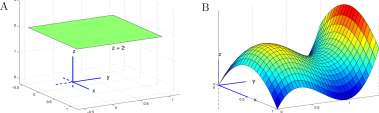
Figure 13.1: Graph in 3-dimensional space of A. F(x, y) = 2 and B. F(x, y) — x (1 — x) + y (1 — y) 2 .

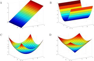
Figure 13.2: Graphs in 3-dimensional space of A. F(x, y) = y, B. Fix, y) = x 2 , C. F(x, y) = x 2 + y 2 , D. F(x,y) = \/x 2 + y 2 –

and aligned so that your thumb lies on and points in the direction of the positive z-axis. Then in a right-handed system, your fingers will point from the positive x-axis to the positive y-axis.

A linear function of two variables is a function of the form F(x, y) = ax + by + c where a, 6, and c are numbers. For example, F(x, y) = 2x + 3y — 6 is a linear function and the graph of 2 = 2x + 3y — 6 in Figure 13.3 is a plane in three-dimensional space. The portion of the graph of z = 2x + 3y — 6 that lies in the plane y = 0 (marked A) is the line z = 2x — 6 in the x, z plane. The x, z plane is the set of all points (x, 0, z) in 3-space. The portion of the graph of z = 2x + 3y — 6 that lies in the plane x = 0 (marked B) is the line z = 3y — 6 in the y, z plane. The portion of the graph of z = 2x + 3y — 6 that lies in the plane z = 0 (marked C) is the line 0 = 2x + 3y — 6 in the (x, y, 0) plane.

CHAPTER 13. TWO VARIABLE CALCULUS AND DIFFUSION

546

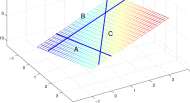
Figure 13.3: Graph of the plane z = 2x + 3y — 6 in three dimensional space. The line marked ‘A’ is the slice of that plane with y = 0. The line marked ‘B’ is the slice with x = 0, and the line marked ‘C is the ‘level curve’ with z = 0.

Definition 13.1.1 Partial Derivative. Suppose F is a function of two variables and (a, b) is in the domain of F. The partial derivative of F with respect to its first variable, denoted by F±, is the ordinary derivative of F with respect to its first variable with the second variable held constant. Similarly, the partial derivative of F with respect to its second variable, denoted by F 2 , is the ordinary derivative of F with respect to its second variable with the first variable held constant.

Second order derivatives are denoted by F it i, F 12 , F 2;1 , and F 22 where F^ is the derivative of Fj with respect to the jth variable.

The limit definitions of partial derivatives are F(a + h,b) – F(a,b)

Fi(a, b) = lim

h

F 2 (a, b) = lim

h— >0

F(a,b + h) – F(a,b)

h

:i3.1)

The Leibnitz notation can be particularly helpful in writing partial derivatives of F(x,y).

dF dF Fi(a,b) =—(a,b), F 2 (a,b) = —(a,b),

d 2 F d 2 F d 2 F

Fi,i(a,b) = —-2-(a,6), F 1>2 (a, b) = —— -(a, 6), F 2i2 (a, 6) = —^(o, 6). ox oyox oy

When notations for the domain variables of F are clear, as in F = F(x, y) it is helpful to write,

for examples,

Fi(x,y) = F x (x,y), F 2 (x,y) = F y (x,y),

and

F lt i(x,y) = F xx (x,y), F 2 ,i(x,y) = F yx (x,y).

CHAPTER 13. TWO VARIABLE CALCULUS AND DIFFUSION

547

Some examples of partial derivatives are: F(x,y) = x 2 + y 2

= 2x F h2 (x,y) = 0 F 2 (x,y) = 2y

F ltl (x,y) = 2 F 2tl (x,y) = 0 F 2a (x,y) = 2

F(x,y) = xe y

2

= e”^ 2 Fi, 2 (a;,|/) = e”f (-2y) F 2 (x,y) = xe~^ {-2y) F ltl (x,y) = 0 F 2tl (x,y) = e’V 2 (-2y) F 2i2 (x,y) = -2x e”» 2 + 4xy 2 e”» 2

F(x,y) = sin(x + y)

F x {x,y) = cos(x + y) F xy (x,y) = -sm(x + y) F y (x,y) = cos(x + y)

F xx {x,y) = -sin(x + y) F yx (x,y) = -s’m(x + y) F yy (x,y) = -sin(x + y)

F(x,y) = x 1 / 2 lny

= (V2)x-V2l n2/ ^|X^) = (i/ 2 ) x -i/2 y -i ^lll = x l/2 y -l

ax w / y axay w 7 y ay w

= -(l/4)s-3/’lny = (l/2),-‘V = -xV V 2

In all of these cases, and usually, F i}2 = F 2>i . Always when Fi >2 and F 2>i are continuous they are equal.

Definition 13.1.2 Limit and continuity of a function of two variables.

Suppose F is a function of two variables with domain D and (a, b) is a point of D and for every positive number 5 there is a point (x,y) of D such that 0 < \J(x — a) 2 + (y — b) 2 < 5, and L is a number. Then

(x,j/)-t-(a,6)

means that if e is a positive number, there is a positive number 5 such that if

(x, y) is in D and 0 < y (x — a) 2 + (y — b) 2 < 5 then \F(x, y) — L\ < e. The statement that F is continuous at (a, b) means that

lim = F(a, 6)

(x,j/)-»(a,6)

or that there is a number Sq > 0 such that for every point (x, y) of -D distinct from (a, 6), y^z – a) 2 + (y – b) 2 > 5 0 .

Explore 13.1.1 Identify the points of the graphs in Explore Figure 13.1.1 A and B at which the graphs are discontinuous.

CHAPTER 13. TWO VARIABLE CALCULUS AND DIFFUSION

548

Explore Figure 13.1.1 A. F(x,y) = 1 if x 2 < y; else F(x,y) = 0.

B. F(x, y) = -(1 + x/2) sin(7ry/2) for x < 0 and -2 < y < 0, y) = (1 – x/2) sin(7r?//2) for x > 0 and -2 < y < 0.

A

B

15 2 -2

In Figure 13.4, slices of the graph of

F(x,y) =x(l-x) 2 +y 2 (l-y)

corresponding to x = 0.2 and y = 0.4 are shown. The line tangent to the slice x = 0.2 at the point (0.2, 0.6, 0.0.432) is drawn. Its slope is

F 2 (0.2,0.6)= 0 + 2y{l-y)-y’

0.12.

Or,y)=(0.2,0.6)

The line tangent to the slice y = 0.4 at the point (0.4, 0.4, 0.24) is also drawn. Its slope is

Fi(0.3, 0.4) = (1 – xf – 2x{l – x)

(x,y)=(0. 4,0.4)

-0.12

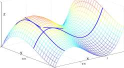
Figure 13.4: Graph in 3-dimensional space of F(x, y) = x(l — x) 2 + y 2 (l — y) and slices through the graph at x — 0.2 and y = 0.4. Observe that this is still a righthanded system although the x- and y-axes are not the same as in previous graphs.

CHAPTER 13. TWO VARIABLE CALCULUS AND DIFFUSION

549

Definition 13.1.3 Local linear approximation, tangent plane. Suppose F is a function of two variables, (a, h) is a number pair in the domain of F, and F\ and F 2 exist and are continuous on the interior of a circle with center (a, b). Then the local linear approximation to F at (a,b) is the linear function

L(x, y) = F{a, b) + F x {a, b) (x – a) + F 2 (a, b) (y – b) (13.2)

The graph of L is the tangent plane to the graph of F at (a, b, F(a, b)), and F is said to be differentiate at (a, b).

For F(x,y) = x 2 + y 2 , Fi(x,y) = 2x, and F 2 (x,y) = 2y. At the point (1,2), F\ and F 2 are continuous on the circle of radius 1 and center (1,2) (actually continuous everywhere), and

F(l, 2) = 5, F t (l, 2) = 2x\ x=ljy=2 = 2, F 2 (l, 2) = 4,

The local linear approximation to F at (1,2) is

L(x, y) = 5 + 2(x – 1) + 4(y – 2).

A graph of F and L appear in Figure 13.5. The graph of L is below the graph of F except at the point of tangency, (1,2,5).

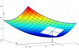
Figure 13.5: Graph in 3-dimensional space of z = F(x, y) = x 2 -\-y 2 and a square lying in the tangent plane at (1,2,5), L(x, y) = 5 + 2(x — 1) + A(y — 2), which is below the graph of F except at the point of tangency, (1,2,5). View is from below the graph. Is this a righthanded axis system?

For a function, F(x,y), of two variables to have a tangent it is necessary that Fi(x,y) and F 2 (x,y) be continuous. For functions / of one variable, the tangent line to the graph of / at (a, f{a)) is simply the line y = f(a) + f'(a)(x — a); f'{a) must exist, but there is no requirement

CHAPTER 13. TWO VARIABLE CALCULUS AND DIFFUSION

550

that f'{x) be continuous or even exist for x 7^ a. For functions of two variables to have a linear approximation, more is required. The example,

F(x,y) = yf\xy\

illustrates the need for conditions beyond the existence of F\{a,b) and F 2 (a, b) in order that there be a tangent plane at (a,b, F(a,b)). See Figure 13.6.

For F(x,y) = yj\xy\, F{0,0) = 0

F(x,0) = 0, Fi(0,0) = 0,

F(0,y) = 0, F 2 (0,0) = 0.

so the local linear approximation at (0,0) might be

L(x, y) = 0 + 0 x (x – 0) + 0 x (y – 0) = 0,

the graph of which is the horizontal plane z — 0. However, the slice of the graph through y = x for

A

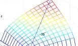
B

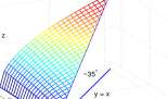
Figure 13.6: A. Graph of F(x,y) = y\xy\ on x > 0, y > 0. The rest of the graph is obtained by rotation of the portion shown about the z-axis 90, 180 and 270 degrees. There is no local linear approximation to F at (0,0) and no tangent plane to the graph of F at (0,0,0). B. Cut away of the graph of A showing the angle between the surface and the horizontal plane above the line y — x.

which z = \x\ shown in Figure 13.6B is a line that pierces the purported tangent plane, L(x,y) = 0, at an angle of about 35 degrees. Thus over the line y = x, L(x, y) = 0 is not tangent to the graph of F. We do not accept the graph of L(x, y) as tangent to the graph of F. Also, F is not differentiate at (0,0). In this case

Fi{x,y)

\y[

\x\

for x > 0, and

2\

\V\

\X\

for x < 0,

.Fi(0, 0) = 0, and i<i(0, y) does not exist for y 7^ 0

F\ is neither continuous nor even defined throughout the interior of any circle with center (0,0). The conditions of Definition 13.1.3 for a local linear approximation are not met.

Explore 13.1.2 Compute F 2 (x,y) for F(x) with center (0,0)?

CHAPTER 13. TWO VARIABLE CALCULUS AND DIFFUSION

551

Property 13.1.1 A property of tangents to functions of one variable. Suppose / is a function of one variable and at a number a in its domain, f'(a) exists. The graph of L(x) = f(a) + f'(a)(x — a) is the tangent to the graph of / at (a, /(a)). Then

lim

x^a

\f(x)-L(x)\

\x — a

lim

x^a

f( x )-f(a)-f(a)(x-a)

x — a

lim f{x) ~ /(a) – /'(a)

x — a

(13.3)

0.

It is sometimes said that the numerator, f(x) — L(x), in

\f(x)-L(x)\

\x

‘goes to zero faster’ than

does the denominator, \x — a\. It is this property that is the defining characteristic of ‘tangent’. Only the existence of f'(a) is required. It is not required that f'(x) be continuous.

As was apparent in Figure 13.5B for the function F(x,y) = \f\xy\, something more than existence of Fi(a,b) and F 2 (a,b) is required in order to have a tangent plane for F(x,y) at a point (a, b). A sufficient condition is that F\ and F 2 exist and be continuous on a circle with center (a, b).

Property 13.1.2 A property of local linear approximations to functions of two variables. Suppose F is a function of two variables, (a, b) is a number pair in the domain of F, and F\ and F 2 exist and are continuous on the interior of a circle with center (a, b). Then L(x, y) = F(a, b) + Fi(a, b)(x — a) + F 2 (a, b)(y — b) is the local linear approximation to F at (a, b), and

lim \ F ^V) – L{x,y)\ =Q (x,y)^(a,b) J( x _ a y + ( y _ h y

The graph of L is the tangent plane to F at the point (a, b, F(a, b)).

The proof of Property 13.1.2 involves some interesting analysis that you can understand, but is long enough that we have not included it. We use this property in proving asymptotic stability of systems of difference equations in Chapter 16.

Exercises for Section 13.1, Partial derivatives of functions of two variables.

CHAPTER 13. TWO VARIABLE CALCULUS AND DIFFUSION 552 Exercise 13.1.1 Draw three dimensional graphs of

Exercise 13.1.2 Find the partial derivatives, F\, F 2 , F± t i, Fi j2 , F 2 ,i and F 2i2 of the following functions.

Exercise 13.1.3 Is the plane z = 0 a tangent plane to the graph of F(x,y) = \/x 2 + y 2 shown in Figure 13.2D.

Exercise 13.1.4 Find F 1 (a,b) and F 2 (a,b) for

a. F(x,y) = I ^ l (a, b) = (1,0)

b. F(x,y) = V^+¥ M) = (1,2)

c. F(x,y) = e~ xy (a, 6) = (0,0)

d. F(x,y) = sin x cosy {a,b) = (7r/2,7r)

Exercise 13.1.5 Find the local linear approximation, L(x,y), to F(x,y) at the point (a,b). For each case, compute

I 7 ‘(•<■■<;)-£(•<■■ .7)1 |ol . (^^ = (0 + 0.1,6), and (x, y) = (a + 0.01, b + 0.01).

CHAPTER 13. TWO VARIABLE CALCULUS AND DIFFUSION

a. F(x,y) =4x + 7y- 16 (a, b) = (3,2)

b. F(x,y)=xy (a, b) = (2,1)

c. F(x,y) = f fj (a, 6) = (1,0)

d. F{x,y)=xe’ y (a, 6) = (1,0)

e. F(z,y) =sin7r(a; + y) (a, 6) = (1/2,1/4)

Exercise 13.1.6 For P = nRT/V, find ^-P and -§fP- For fixed T, how does P change as V increases? For fixed V, how does P change as T increases?

Exercise 13.1.7 Draw the graph of F(x ) y) and the graph of the plane tangent to the graph of at the point (a,b). A MATLAB program to solve c. is shown in the answer to this exercise, Exercise 13.1.7.

Exercise 13.1.8 Let F be defined by

F(x, y) = x 2 for y > 0

= 0 for y < 0

1. Sketch a graph of F in three dimensional space.

2. Is Fi(x,y) continuous on the interior of a circle with center (0,0)?

3. Let L(x,y) = 0 for all (x,y). Is it true that

hm ^4 ‘ L(X,y) = 0 ?

(x,y)->{0,0) L.2 _^ y2

4. Are you willing to call the plane z = 0 a tangent plane to the graph of Fl

CHAPTER 13. TWO VARIABLE CALCULUS AND DIFFUSION

554

13.2 Maxima and minima of functions of two variables.

Figure 13.7B shows a slice of the graph of F(x, y) = x(l — x) 2 + y 2 (l — y) through x — 1/3 and a slice through y = 2/3. The point (1/3, 2/3, 8/27) at which these slices intersect appears to be and is a local maximum for F. The two tangents to these slices are horizontal as would be expected at an interior local maximum for a function of a single variable. The point (1/3,2/3) and associated slices were selected by solving two equations for x and y:

Fx(x,y) = l-4x + 3x 2 = 0

F 2 (x,y) = 2y-3y 2 = 0. There are four solutions, called critical points of F,

(x,y) = (1/3,2/3), (x,y) = (1/3,0), (x, y) = (1, 2/3) and (x,y) = (1, 0).

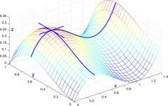
Figure 13.7: Slices through the graph of F(x,y) = x(l — x) 2 + y 2 (1 — y) through x = 1/3 and y = 2/3. (1/3,2/3,8/27) is a local maximum of F.

Definition 13.2.1 Critical points. A point (a, b) of the domain D of a function of two variables, F, is an interior point of the domain if there is a circle centered at (a, b) whose interior is a subset of D. Points of D that are not interior points are called boundary points of D.

An interior point (a, b) of F is a critical point of F means that

F 1 {a,b) = 0 and F 2 {a,b) = 0

or that one of Fi(a, b) or F 2 (a, 6) fails to exist. Boundary points of D are also critical points of F.

CHAPTER 13. TWO VARIABLE CALCULUS AND DIFFUSION

555

There are four critical points of F(x, y) = x(l — x) 2 + y 2 (l — y),

(1/3,2/3), (1,2/3), (1/3,0), and (1,0).

The critical point (1/3,2/3) is discussed above and shown in Figure 13.7.

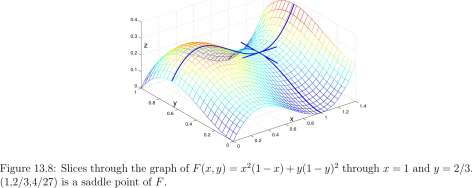
The critical point (1,2/3) is illustrated in Figure 13.8 and is neither a high point nor a low point, it is a saddle point. The surface is convex upward in the x-direction and is concave downward in the ^-direction. The tangent at (1,2/3,4/27) parallel to the y-&xis is above the surface; the tangent parallel to the x-axis is below the surface and would normally not be visible.

The critical point (1,0) is illustrated in Figure 13.9 and is a local minimum for F and is illustrated in Figure 13.9. The domain for y is [-0.4,1]; in Figures 13.7 and 13.8 the domain for x is [0,1]. Also the viewpoint is lower in Figure 13.9 than in Figures 13.7 and 13.8 in order to look underneath the graph at the low point.

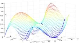
Figure 13.9: Slices through the graph of F(x,y) = x(l — x) 2 + y 2 {l — y) through x = 1 and y = 0. (1,0,0) is a local minimum of F.

A

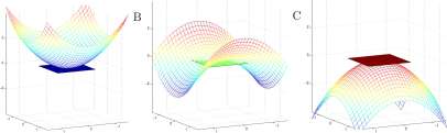
Figure 13.10: Graphs of A. z = x 2 + y 2 , B. z = x 2 — y 2 , and C. z = —x 2 — y 2 . The local linear approximation to each is the horizontal plane z = 0.

Explore 13.2.1 Locate the critical point (1/3,0) of F(x,y) = x(l — x) 2 + y 2 (l — y) in Figure 13.9 and classify it as a local maximum, local minimum or saddle point. ■

Example 13.2.1 The graphs of F(x, y) = x 2 + y 2 , G(x, y) = x 2 — y 2 and H(x, y) = —x 2 — y 2 shown in Figure 13.10 illustrate three important options. The origin, (0,0), is a critical point of each of the graphs and the z = 0 plane is the tangent plane to each of the graphs at (0,0). For F, for example,

F(x,y) = x 2 + y 2 Fi(x,y) = 2x F 2 (x,y) = 2y

F(0,0) = 0 ^i(0,0) = 0 F 2 (0,0) = 0

The origin, (0,0), is a critical point of F, the linear approximation to F at (0,0) is L(x, y) = 0, and the tangent plane is z = 0, or the x, y plane. The same is true for G and H; the tangent plane at (0,0,0) is z = 0 for all three examples. This seemingly monotonous information is saved by the observations of the relation of the tangent plane to the graphs of the three functions. For F, (0,0,0) is the lowest point of the graph of F, and for H, (0,0,0) is the highest point of the graph of H. This is similar to the horizontal lines associated with high and low points of graphs of functions of one variables. The graph of G is different. The point (0,0,0) is called a saddle point of the graph of G. The portion of G in the x, z plane (y = 0) has a low point at (0,0,0) and the portion of G in the y, z plane (x = 0) has a high point at (0,0,0).

For a function / of a single variable and a number a for which f'(a) = 0, there is a simple second derivative test, Theorem 9.2.3, that distinguishes whether (a, f(a)) is a locally high point (/”(a) < 0 ) or a locally low point (/”(a) > 0 ). There is also a second derivative test for functions of two variables.

Definition 13.2.2 Definition of Local Maxima and Minima. If (a, b) is a point in the domain of a function F of two variables, F(a, b) is a local maximum for F means that there is a number So > 0 such that if (x, y) is in the domain of F and yj(x – a) 2 + (y – b) 2 < S 0 then F(x, y) < F(a, b).

The definition of local minimum is similar.

CHAPTER 13. TWO VARIABLE CALCULUS AND DIFFUSION

557

Theorem 13.2.1 Local Maxima and Minima of functions of two variables.

Suppose (a, b) is a critical point of a function F of two variables that has continuous first and second partial derivatives in a circle with center at (a, b) and

A = F lil (a,b)F 2i2 (a,b)-(F 1 , 2 (a,b)) 2 .

Case 1. If A > 0 and F^i (a, b) > 0 then F(a, b) is a local minimum of F.

Case 2. If A > 0 and F^i{a, b) < 0 then F(a, b) is a local maximum of F.

Case 3. If A < 0 then (a, b, F(a, b)) is a saddle point of F.

Case 4. If A = 0, punt, use another supplier.

We omit the proof of Theorem 13.2.1, but illustrate its application to the functions F, G, and H of Example 13.2.1 and shown in Figure 13.10.

For F{x,y) = x 2 + y 2 , A = 2×2-0 = 4>0, Fi,i(0, 0) = 2 > 0,

and the origin is a local minimum for F.

For G(x,y) = x 2 -y 2 , A(0, 0) = 2 (-2) – 0 =-4 < 0,

and the origin is a saddle point for G. We have not defined a saddle point. For our purposes, a saddle point is a critical point for which A < 0.

For H(x,y) = -x 2 -y 2 , A =-2 (-2) – 0 = 4 > 0, # 1;1 (0, 0) = -2,

and the origin is a local maximum for H.

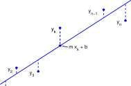
Example 13.2.2 Least squares fit of a line to data. A two variables minimization problem crucial to the sciences is the fit of a linear function to data.

Problem. Given points (x 2 ,y 2 ), • • •, (x n ,y n ), where X; L ^ Xj if i ^ j, find numbers a 0 and b 0

so that (a, b) = (a 0 , b 0 ) minimizes

n

SS(a, b) = J2 (Vk-a- bx k f (13.5) k=i

In Figure 13.2.2.2, SS(a,b) is the sum of the squares of the lengths of the dashed lines.

Figure for Example 13.2.2.2 A graph of data and a line. SS(a,b) is the sum of the squares of

the lengths of the dashed lines.

CHAPTER 13. TWO VARIABLE CALCULUS AND DIFFUSION

558

m x, + b

k

n-1 n

Solution. The critical points of SS are the solutions to the equations

SSU^b) = –SS = 0 SS 2 (a,b) = ^-SS = 0. da ” do

(13.6)

SS\(a, b)

d_ da

Y (Vk-a- bx k )

k=i

t ~(y k -a-bx k f

k=l

= 2 (y k – a – bx k ) (-1)

k=l n

= 2 J2 ( a + bx k ~ Vk) k=l

2[aJ2 l + b^2 x k -J2 Vk

k=l k=l

k=l

SS 2 (a, b)

d db

Y (Vk ~ a ~ bx kY

k=l

d

Y ^ Vk ~ a ~ bXk ^ 2

k=l

Y 2(y k -a- bx k ) {-x k )

k=i

2 Y (ax k + bx\ – x k y k J

k=l

= 2 laY x k + bJ2 s l~Y x kVk)

\ fc=l k=l k=l /

Imposing the conditions SS\(a, b) = 0 and SS^a, b) = 0 and simplifying leads to the Normal Equations:

an + b ELi x k = Efc=i Vk a ELi x k + b ELi x fc = Efc=i ^

(13.7)

CHAPTER 13. TWO VARIABLE CALCULUS AND DIFFUSION

559

Some notation is useful:

n n n n n

= = Vkt = X k , S X y = Xfc l/f., Syy = .

k=l k=l k=l k=l k=l

The solution to the Normal Equations 13.7 is

Q Q — Q Q

‘-‘xx u y “-‘x’-‘irt/

Q.Q

~A

a

:i3.8)

A = nS xx – (S x )

It is important that A^O. The proof that A is actually positive involves some clever and not very intuitive algebra. Form the sum

S — (S xx S x Xk) ■

k=l

Because the x^ are distinct, at least one of S xx — S x Xk ^ 0 and S > 0.

n

S — J]] {Sxx ~ S x Xk)

fc=l

{{Sxx) 2S XX S X Xk + {S;

fc=l

{Sxx) %S XX S X Xk + {s x ) 2

k=l k=l k=l

n {S X x) ~ 2S XX S x S x + {Sx) S xx Sxx{f^S xx {S x ) )

x k

— S X x A

Now S xx > 0 and S = S xx A > 0, so A > 0. Explore 13.2.2 Why is S xx positive? m

Example 13.2.3 Fit a line to the data in Example Figure 13.2.3.3. Figure for Example 13.2.3.3 Data, a graph of the data and a line y = a + bx fit to the data:

CHAPTER 13. TWO VARIABLE CALCULUS AND DIFFUSION

560

S x = 1 + 2 + 4 + 6 + 8 = 21,

S y = 0.5 + 0.8 + 1.0 + 1.7+1.8 = 5.8

Sxx = l 2 + 2 2 + 4 2 + 6 2 + 8 2 = 121,

S xv = 1-0.5 + 2 -0.8 + 4- 1.0 + 6 -1.7 + 8 -1.8 = 30.7

A = n S xx – (S x ) 2 = 5 • 121 – (21) 2 = 164 a = (S xx S y – S x S xy )/A = (121 ■ 5.8 – 21 ■ 30.7)/164 = 0.348 b = (nS xy – S x S y )/A = (5 • 30.7 – 21 • 5.8)/164 = 0.193

The line y = 0.348 + 0.193a; is the closest to the data in the sense of least squares and is drawn in Example Figure 13.2.3.3.

You would systematically organize the arithmetic if you fit very many lines to data as we just did. Better than that, the following MATLAB commands do the same task for the data in Example Figure 13.2.3.3.

close all;clc;clear I plot(x,y, ‘o’, , linewidth J ,2)

x=[l 2 4 6 8]; y=[0.5 0.8 1.0 1.7 1.8]; I hold(‘on’) P=polyfit(x,y,1) I plot(xp,yp,’linewidth ) ,2)

xp=[0.5 8.5]; yp=polyval(P,xp); I

Furthermore, there are many programmable hand calculators that will do this task. What is required is that you load the data in two vectors or lists, find the coefficients of the line closest (in the least squares sense) to the data, plot the data and plot the line.

Example 13.2.4 Problem: Find the dimensions of the largest box (rectangular solid) that will fit in a hemisphere of radius R.

Solution. Assume the hemisphere is the graph of z — \/R 2 — x 2 — y 2 and that the optimum box has one face in the x,y-p\ane and the other four corners on the hemisphere (see Figure 13.2.4.4).

Figure for Example 13.2.4.4 A. A box in a hemisphere. One corner of the box is at (x,y) in the x, y-plane. B. Graph of W(x, y) = max(0, x 2 y 2 (1 — x 2 — y 2 ))-

A

B

0.035

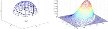
The volume, V of the box is

V(x, y) = 2x x 2y x z = 4 x y JR 2 — x 2 — y 2

CHAPTER 13. TWO VARIABLE CALCULUS AND DIFFUSION

561

Before launching into partial differentiation, it is perhaps clever, and certainly useful, to observe that the values of x and y for which V is a maximum are also the values for which V 2 /16 is a maximum.

y2 ( x ,y) \xt ( \ ^x 2 y 2 (R 2 -x 2 -y 2 )

W(x,y)

16 v ia ‘ 16

It is easier to analyze W(x,y) than it is to analyze V(x,y).

Wx(x,y) = 2R 2 xy 2 – Ax 3 y 2 – 2xy A

r>2 2 2 4 2 2 4

R x y — x y — x y .

2xy 2 (R 2 – Ax 2 – 2y 2 )

W 2 (x,y) = 2R 2 x 2 y – 2x 4 y 2 – Ax 2 y 3

2x 2 y{R 2 – 2x 2 – Ay 2

Solving for W 1 (x,y) = 0 andW / 2 (x,?/) = 0 yields x = R/^/3 and y = R/V3, for which z = R/y/3. The dimensions of the box are 2 J R/v / 3, 2i?/\/3, and R/V3.

Explore 13.2.3 Are there some critical points of W other than (R/y/3, R/J(3), R/y/3)? h Example 13.2.5 Warning: Obnubilation Zone. Problem. Find the point of the ellipsoid

2 2 2

\ + \ + — = 1 that is closest to (-2,3, -1) (13.9) 14 9

See Example Figure 13.2.5.5

Figure for Example 13.2.5.5 The ellipsoid x 2 /l + y 2 /A + z 2 /9 = 1 and a line from (-2,3,-1) to a

point (x,y,z) of the ellipsoid.

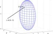
Solution. Claim without proof: The point (x, y, z) of the ellipsoid that is closest to will have negative x, positive y, and negative z coordinates.

The distance between (a, b, c) and (p, q, r) in 3-dimensional space is

-2,3,-1)

^J(p-ay + (q-by + (r-cy. The distance from (-2,3,-1) to (x,y, z) on the ellipsoid is

CHAPTER 13. TWO VARIABLE CALCULUS AND DIFFUSION

We solve for z in Equation 13.9 and write

z = —3\Jl — x 2 — y 2 /4 z is negative.

E(x,y) = ] /(x + 2) 2 + ( y – 3)2 + (1 – x 2 – y 2 /4) 2

Define F(x,y) = (E(x,y)) 2 and write

F(x,y) = (x + 2) 2 + (y- 3) 2 + (l – 3^1 – x 2 – y 2 /A^

F 1 (x,y) = 2{x + 2) + 2 (l – 3^1 – x 2 – y 2 /^j |- (l – 3^1 – x 2 – y

= 2(x + 2) + 2 ( 1 – 3Jl -x 2 – y 2 /4) —t

v ; 20T

F 2 (a;,y) = 2(y – 3) + 2 f 1 + 3^1 – x 2 – y 2 /4]

V v / 2^1 – – y 2 /4

Now we have a mess. We need to (and can!) solve for (x,y) in

Fx(x,y) = 2(x + 2) + 6x I 1 – 3 = 0

; -3)(-2x) — x 2 — y 2 /4

3(-2y/4)

F 2 (x,y) = 2(y-3) + f I , 1 -3

First we write

2(x + 2) = -6x

2fe-3) = -f

divide corresponding sides of the two equations, and find that

12x V ~ 3a;-2′

Substitute this expression for y in Equation 13.12, simplify, and find that

o x o T3s(3s-2)

^(1 – x 2 )(9x 2 – 12x + 4) – 36a; 2 Square both sides of this equation and clear fractions.

(8x – 2) 2 [(1 – a; 2 ) (9a; 2 – 12x + 4) – 36a; 2 ] = 9x 2 (9x 2 – 12a; + 4) Multiply and collect.

576a; 6 – 1056a; 5 + 2485x 4 – 380a; 3 – 480a; 2 + 176a; – 16 = 0 Now we have it! In MATLAB issue the two commands,

CHAPTER 13. TWO VARIABLE CALCULUS AND DIFFUSION

563

format long and roots([576 -1056 2485 -380 -480 176 -16])

The output will be

0.793717568921366 + 1.862187416061669i 0.793717568921366 – 1.862187416061669i -0.482870021732987 0.281691271346906 + 0.0743913583599971 0.281691271346906 – 0.074391358359997i 0.165385674529775

Many programable hand calculators have polynomial root solving capabilities also.

There are two real roots, -0.482870021732987 and 0.165385674529775. Use x = 0.165385674529775 and compute y = 1.680224831 and z = -0.726205610 from Equations 13.13 and 13.10, and the distance from (-2,3,-1) to the ellipsoid is 2.029. Whew!

Explore 13.2.4 For the algebraically strong, fill in the algebra omitted in Example 13.2.5

Exercises for Section 13.2 Maxima and minima of functions of two variables. Exercise 13.2.1 Find the critical points, if any, of F.

Exercise 13.2.2 For each of the following functions, find the critical points and use Theorem 13.2.1 to determine whether they are local maxima, local minima, or saddle points or none of these.

Exercise 13.2.3 Find C and b so that Ce bx closely approximates the data

CHAPTER 13. TWO VARIABLE CALCULUS AND DIFFUSION

564

Observe that for y = Ce bx , Iny = InC + bx. Therefore, fit a + bx to the number pairs, (x, Iny) using linear least squares. Then Inyk = a + bxk, and

y k = e *+b*k = e *. e bxk =Ce bx \ where C = e a .

Exercise 13.2.4 a. Find a, b, and c so that y = a + bx + cx 2 is the least squares approximation to data, (xi,yi), x 2 ,y2), • • •, (x n ,y n ). To do so you will need to minimize

n 2

SS = J2 (yk – (a + bx k + cxlf) . fc=i

This is a three-variable minimization problem. The solution will be similar to the least squares line approximation to data of Example 13.2.2. b. In Exercise Table 13.2.4 are data showing the height of a ball falling in air above a Texas Instruments CBL motion detector. Find the parabola that is the least squares fit to the data, c. Check your answer on a computer or calculator.

Table for Exercise 13.2.4 Height of a ball falling in aire above a Texas Instruments CBL motion

detector.

Time; sec 0.232 0.333 0.435 0.537 0.638 0.739 0.840 Position cm 245.9 235.8 214.3 184.1 146.0 99.3 45.5 Exercise 13.2.5 Find a and b so that sin(ax + b) closely approximates the data

Observe that for y = sin(a:r + b), arcsiny = ax + b. Therefore, fit ax + b to the number pairs, (x,arcsiny) using linear least squares.

Exercise 13.2.6 Interpret the real root x = 0.165385675 of Equation 13.14 related to the ellipsoid example.

Exercise 13.2.7 Find the largest box that will fit in the positive octant (x > 0, y > 0, and z > 0) and underneath the plane z — 12 — 2x — 3y.

Exercise 13.2.8 Find the largest box that will fit in the positive octant and underneath the hemisphere z = — x 2 — y 2 .

Exercise 13.2.9 Find the point of the plane z = 2x + 3y — 12 that is

1. closest to the origin.

2. closest to (4,5,6)

CHAPTER 13. TWO VARIABLE CALCULUS AND DIFFUSION

565

Exercise 13.2.11 Find the point of the ellipsoid of Equation 13.9

2 2 2

%- + V — + — = 1 that is farthest from (-2,3, -1) (13.15) 14 9

Exercise 13.2.12 In Exercise 8.3.3 1 we found that the average power over a whole cycle of a bounding flight of a bird should be

2 2

P = (1 – x)P fo i ded + xP flappin g = A b U 3 + xA w U 3 + B

XU

where and A& + A w are, respectively, drag coefficients of the bird without wings extended and with wings extended and flapping, B is a constant, u is the speed of flight, m is the mass of the bird, g is the acceleration of gravity, and x is the fraction of a flight cycle during which the wings are flapping. You were to find the fraction, x, for which the required power is a minimum and the fraction, x, for which the required energy is a minimum, with E = P/u. You may have found that x = A w /Bmg/u 2 for both answers.

Find, if there is one, the combination of flight speed, u, and fraction x for which the power P is a minimum.

Find, if there is one, the combination of flight speed, u, and fraction x for which the energy E is a minimum.

13.3 Integrals of functions of two variables.

Suppose F(x,y) is a positive function of two variables defined on a region R of the x,y-plane. What is the volume, V, of the region above the x,y-plane and below the graph of z — F(x,y)7 (Figure 13.11A.)

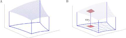
Figure 13.11: A. Graph of a function F of two variables and the region between the graph and the x,y-plane. B. The domain of F is partitioned into small regions.

The volume can be approximated as follows. (Figure 13.11)

Step 1. Choose a positive number 6 and partition R into regions Ri, R2, ■ ■ ■, R n of diameter less than 5.

1 Analysis based on R. McNeill Alexander, “Optima for Animals” Princeton University Press, Princeton, NJ, 1996, Section 3.1, pp 45-48.

CHAPTER 13. TWO VARIABLE CALCULUS AND DIFFUSION

566

Step 2. Let P; be a point in R i} i — 1, • • •,n, and let Ai be the area of R{. Step 3. Then

V = J2F{Pi)A (13.16)

The approximation 13.16 converges to V as 5 —> 0.

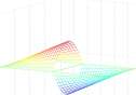
The graph of F(x,y) = (sin7rx) (cos |?/) is shown in Figure 13.12 with the domain 0 < x < 1, 0 < y < 1 partitioned into 25 squares of sides 0.2 and a point marked at the center of each square. The volume of the region below the graph of F and above the x, y-plane is approximately

4 4

sin((0.1 + i ■ 0.2) • vr) cos((0.1 + j ■ 0.2) • (tt/2)) x 0.2 x 0.2 = 0.414

i=0 j=0

Similar computations with 100 squares of sides 0.1 yields 0.407 as the approximate volume and with 400 squares of sides 0.05 yields 0.406.

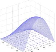
Figure 13.12: The graph of F(x,y) = (sin7ra;) (cos |y) on 0 < x < 1, 0 < y < 1. The domain is partitioned into squares and the center point of each square is marked.

The sum in Equation 13.16 has other applications than approximating volumes and the following definition is made.

Definition 13.3.1 Integral of a function of two variables. Suppose F is a continuous function defined on a region R of the x, y-plane. The integral of F on R is denoted and defined by

jj F{P)dA = \imj2F{P l )A l where S, n, Pi and Ai are as in Steps 1 and 2 above.

(13.17)

CHAPTER 13. TWO VARIABLE CALCULUS AND DIFFUSION

567

The word “region” has been used without definition and ambiguously. We have written of regions in three dimensional space below the graph of a function of two variables and regions in the £,2/-plane. We could write “3d-region” and “2d-region” to clarify at least the context. If you approximate the integral of a function of two variables, you are well advised to choose “simple” regions in the x, y-p\ane whose easily computed. Rectangles plus their interior are good.

In Example 13.3.2 we use sectors of annular rings which are polar coordinate “rectangles.” We rely on your good will to use the word “region” ambiguously and without formal definition.

Suppose now that R is the region in the x, ?/-plane between the graphs of two functions / and g of a single variable defined on an interval [a, b] as shown in Figure 13.13A. (R is the set to which (x, y) belongs only if a < x < b and f(x) < y < g{x)).

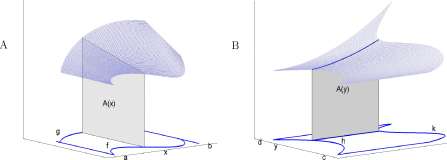
Figure 13.13: A. The domain of F is the set of (x,y) for which a < x <b and f(x) <y< g{x). B. The domain of F is the set of (x, y) for which c < y < d and h(y) < x < k(y).

Then for each number x in [a, b] the area of the cross section through V at x is

/■g( x )

A(x) = / F(x, y) dy

Using the volume equation 11.2, the volume V is

V = J A(x) dx = J ^ j F(x, y) dy^j dx

Alternatively, Figure 13.13B, there may be two functions h(y) and k(y) defined on an interval [c, d] and R is the region to which (x, y) belongs only if c < y < d and h(y) < x < k(y). Then

v = Ic ( Ik”) F ^ y “> dx ) dy

More generally, two ways to compute the integral of F(P) are

( f F(P)dA= [ b f 9(X) F(x,y)dydx (13.18)

JrJ J a Jf(x)

CHAPTER 13. TWO VARIABLE CALCULUS AND DIFFUSION

568

and

R

-d rk(y)

F(P)dA = I / F(x,y)dxdy.

Jh{y)

13.19)

In the ‘inside’ integration F(x,y) dy of Equation 13.18, x is a constant, the integration is with

respect to the variable y. Similarly, in the integration F(x,y) dx of Equation 13.19, y is a constant, the integration is with respect to the variable x.

Example 13.3.1 The domain of the function F(x,y) = (sin7rx) (cos |y) shown in Figure 13.12 is 0 < x < 1, 0 < y < 1. Choose f(x) = 0 and g(x) — 1, for 0 < x < 1. The volume of the region below the graph of F is

7T

1 f 1

/ (sin ttx) (cos —y) dy dx o Jo 2

i

o

2 r l

IT JO

2 2

7T 7T

7T

(sin7rx) (sin —y) x

2 71

sin 7ix dx

2″iv=i

= 0.405285

Problem. Find the volume, V, of the three dimensional region below the graph of z = 1 + 2x/3 + y/3 and above the triangle bounded by x = 1, y — 1 and x + y — 4. (Figure 13.14.)

3-

A

B

y 1

0 0

Figure 13.14: A. The region, R, bounded by the graphs of x — 1, y = 1, and a; + y = 4. B. The three-dimensional region above R and below the graph of z — 1 + 2x/3 + y/3.

CHAPTER 13. TWO VARIABLE CALCULUS AND DIFFUSION

569

Solution. Define f(x) = 1 and g(x) = 4 — x for 1 < x < 3. V = J? ft x (l + 2x/3 + y/3)dydx

Ii

y + (2x/3)y + \

6

y=4:—x

dx

y=l

Si (4-x) + (2x/3)(4-x) +

(4 – xf

-(l + (2x)/3-^ dx

ii T

~T X

6 X

Problem. Find the volume, V, of the three dimensional region below the graph of z = 1 — xy and above two dimensional region R bounded by y — —\/x, y = \fx and x = 1.

Solution 1. Define f(x) = —y/x and g(x) = \/x for 0 < x < 1. (Figure 13.15A.)

A

B

C

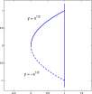
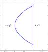
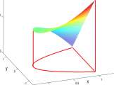
Figure 13.15: A. The region can be defined by 0 < x < 1, —V^c < y < y/x or B. by —1 < y < 1, < x < 1.

^ = Jo 1 Ivi (l-xy)dydx

ll

Jq 1 2 rfx

x

3/2

3/2

4 3

CHAPTER 13. TWO VARIABLE CALCULUS AND DIFFUSION

570

y 2 < x < 1 for -1 < y < 1. (Figure 13.15B.) Then

V

l\ (l-xy)dxdy

x —

(0 – D

1 1 x=l

x y

dy

x=y z

7/ 2 – y

dy

A ( l ~ y ?-y 2 + i) d y

4 3

Problem. Compute J R J F(P) dA where R is the annular ring 1 < y/x 2 + y 2 < 2. There are several solutions, one of which is illustrated in Figure 13.16. Partition R into four regions, Ri – R4 each of which is in the form a < x < b, f(x) < y < g(x). Then

/ / F{P)dA = [ f F{P)dA+ j [ F(P)dA+ [ j F{P)dA+ [ [ F{P)dA

JR J J Hi J JRo J JRz J JRi J

1 ryJT-

1 fV^t

F(x,y)dydx+ I I F(x,y)dydx +

y/A^X? J-i JVI^x 2

1 r-Vl-x 2 t-2 rVi-x 2

F(x,y)dydx+ / / F(x,y)dydx

-1 J-V4~x 2

1 J-V^Q

-2 -1.5 -1 -0.5 0 0.5 1 1.5 2

Figure 13.16: An annular ring partitioned into four regions.

Example 13.3.2 A clever manipulation. The normal probability density was first defined by A. De Moivre in 1733 as

f(t) = — i =e-( t -^/ 2 ° 2 .

aV2vr

CHAPTER 13. TWO VARIABLE CALCULUS AND DIFFUSION

The coefficient 1/V27T insures that

f° f(t)dt= [°° ^=e~ t2 l 2 dt = lim f -^=e{2 l 2 dt=\

J-oo J-oo Jl-K c ^°° J-c

-oo V27T c ^°° ^-c V27T

This requires, and we wish to prove, that

1= T e~ t2 / 2 dt = V2^

J — oo

The difficulty stems from the lack of an antiderivative formula for / e~* 2 / 2 dt. There is none. However, we write

I 2 = r e’ x2 l 2 dx x r ey2 l 2 dy = /°° (7°° e^dx) e”^ 2 dy

J—oo J —oo J—oo \J — oo /

= r r e-* 2 / 2 e-y’ 2 / 2 dxdy = [ ( e~^l 2 dA

J—oo J —oo JrJ

where R is the x, y-plane.

Now we use a clever approach to the last integral. Label points in the plane with polar coordinates (r, 6) where

r = \J 1 x 2 + y 2 and cos6 = x/r, sm9 — y/r With these coordinates

f(x,y)=g(r,6) = er2 / 2

and we will compute J R J e~ r / 2 dA.

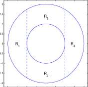
For each positive number c, let R c be the circular region centered at the origin and radius See Figure 13.17. For m and n positive integers, partition [0, c] by = i x c/m, i = 0, m, and [0, 27r] by 9j = j x 2n/n, j = 0, n. R c is partitioned into m x n subregions

Rij = ri-i <r<Ti Oj-i <6<6j

The area of R itj is A itj = (ix (r^) 2 – 7r (rvi) 2 ) x ^ = 27r ? ^L ^tll(r i – r^i) x 1 -Now evaluate e -7 ” 2 / 2 in at Pj = ((rj_i + rj)/2, 0j + 7r/n) and write

Lje-^dA = EE e Jii;c J i=i j=i

((ri_i+ri)/2) 2 /2 4. .

m, n

E E e-«+ -)/ 2 ) 2 / 2 2 7 r^±^(r l -r l _ 1 ) i i=i j=i 2 n

2vrE e-«^)/2)V2 r ^i± rj ( ri – f 1 •=1 2 j=i n

2vrE e-^^^-^^iu-r^) x 1

CHAPTER 13. TWO VARIABLE CALCULUS AND DIFFUSION

572

o

Figure 13.17: A circular region of radius c partitioned into subregions. The shaded subregion is n-i <r<n, B 3 -x <6< 6j.

We conclude that

/ / e~ r2/2 dA = lim / / e~ r2/2 dA= lim 2tt(1 – e” c2/2 ) = 2tt.

JR J c ^°° Jr c J c->oo

Therefore

/oo e~* /2 dt = \/2tt -oo

as was to be proved. ■

Exercises for Section 13.3, Integrals of functions of two variables.

Exercise 13.3.1 Approximate the volume of the region between the graph of F and the x, y-plane using six or more subregions of its domain and a point selected in each subregion.

Exercise 13.3.2 Sketch the domains over which the integrals are defined.

a J? if F(x,y)dydx b ff F(x,y)dxdy c $ J 3 4 F(x,y)dydx

CHAPTER 13. TWO VARIABLE CALCULUS AND DIFFUSION

573

Exercise 13.3.3 Cyclic AMP is released by a slime mold amoeba at the center of a 6 mm by 4 mm flat plate. The concentration at position (x,y) is e~ x +y molecules/mm 2 , where the x-axis runs through the center of the plate in the 6 mm direction, the |/-axis runs through the center of the plate and is perpendicular to the x-axis.

a. Write an integral that is the amount of cyclic AMP released by the amoeba.

b. Compute an approximate value of the integral.

Exercise 13.3.4 Write but do not compute the iterated form of the integral J R J F(P) dA for the functions F and domains indicated. In i. and j. write the integral as the sum of two iterated integrals.

Exercise 13.3.5 Evaluate the integrals.

a- Jo I2 xy 2 dydx b. J 2 4 xy 2 dxdy c. ^ I2 xy 2 dxdy

d. Jo So xy 2 dxdy e. Jq j* 2 xydydx f. J-f ff x 2 + y 2 dxdy

g- Ii Je~* f d y dx h – Jo* Ji~ x2 x + ydydx i. Jq 1 j^Z$ x + ydydx Exercise 13.3.6 Write an integral that is the volume of the region below the graph of

z = 16 — x 2 — 4y 2

and above the x,y-p\ane.

13.4 The diffusion equation u t (x,t) = c 2 ^ x (x,t).

Partial derivatives may appear in equations and when they do the equations are called partial differential equations. This is a vast field of study. We give one very important example, the diffusion equation, and suggest a numerical method for its solution.

CHAPTER 13. TWO VARIABLE CALCULUS AND DIFFUSION

574

The diffusion equation in one space dimension is

u t (x,t) = c 2 u xx (x,t), a < x < b, 0 < t. (13.20)

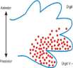
Embryonic digit development On the limb bud of the developing vertebrate embryo, there is a “zone of polarizing activity” (ZMP) on the “pinky” side of the limb bud that causes the pinky side to be different from the thumb side. A protein, sonic hedgehog, is emitted from the ZMP and diffuses across the limb bud. The concentration of sonic hedgehog decreases with the distance from the ZMP; those digits closest to ZMP with high hedgehog protein concentration develop into the pinky and ring fingers; those farthest from the ZMP with low hedgehog protein concentration develop into the index finger and thumb (see Figure 13.18). This extremely important diffusion example is too complex for us to model, and we turn to simpler problems.

Digit I-SHH independent

II-lowSHH concentration

Digit III – bfief SHH expression, high SHH concentration

Digit IV – moderate SHH expression

extended SH H expression • Descendants of SHH expressing cells

Figure 13.18: Sonic hedgehog specifies digit identity in mammalian development. From http://en. wikipedia.org/wiki/Hedgehog_signaling_pathway

u(x, t)

i—

0

x

—i L

You may think of a brass rod of diameter, d, that is small compared to its length, L = b — a, and u(x,t) as the temperature in the rod at position x and at time t. If the temperature is not at equilibrium, the flow of heat in the rod will cause the temperature to equilibrate according to Equation 13.20. For a fixed value, x of x, u(x,t) describes the temperature at position x for times t > 0. For a fixed value, t of t, u(x,t) describes the temperature distribution in the rod at time t.

Alternatively, you may think of a glass tube of diameter, d, that is small compared to its length, L = b — a, and is filled with distilled water with a small amount of salt dissolved in it, and u(x,t) as the concentration of salt at position, x, and time t. If the salt concentration is not at equilibrium, salt will flow in the rod and will cause the concentration to equilibrate according to Equation 13.20.

A single equation describes u(x,t) for both of these problems and a host of other problems. Molecules diffuse in intercellular fluids during embryonic development and within intracellular fluids; diseases diffuse in a population; an invasive species diffuses over an extended range. James D. Murray has shown 2 that a linked pair of reaction-diffusion equations defined on a

2 James D. Murray, How the leopard gets its spots, Scientific American, 1988, 258(3) pp 80-87., James D. Murray, Mathematical Biology, Springer-Verlag, Heidelberg, 1989.

CHAPTER 13. TWO VARIABLE CALCULUS AND DIFFUSION

575

two-dimensional surface can nicely replicate numerous mammalian coat patterns, ranging from the giraffe, leopard, zebra, to the elephant (neutral).

In order to determine u(x,t) it is necessary to know the initial state of u,

u(x,0)=g(x), say,

and the constraints on u(x,t) at the ends of the rod,

u(a,t) = h a (t), and u(b,t) = kbit), for example.

We derive the diffusion equation in terms of the diffusion of salt (or any solute). Consider a circular glass rod of cross sectional area A and length L filled with water and assume that at time t — 0 the concentration of the salt along the tube is g(x). Let u(x,t) be the salt concentration at distance x from one end of the rod at time t. Figure 13.19A. Assume that the diameter of the rod is small enough that the salt concentration at any position x along the rod depends only on x.

u(x,t)

A

B

C

Figure 13.19: A. Glass rod, salt concentration at x at time t is u(x, t). B. The rate at which salt flows past position x is proportional to — u x (x, t). C. The amount of salt between x — d and x + d at time t is approximately u(x,t) x A x 2d.

Diffusion: Mathematical model 1. Salt tends to flow from regions of high concentration to regions of low concentration. The rate at which salt flows past position x in the direction of increasing x at time t is proportional to — u x (x, t) and to A, the cross sectional area of the rod. Figure 13.19B.

From this model we write

R(x,t) = -kAu x (x,t) (13.21)

where R(x, t) is the rate at which salt diffuses past position x at time t and k is a proportionality constant that is a property of the solvent/solute system.

Units. The units on u, u x , A and R are, respectively,

CHAPTER 13. TWO VARIABLE CALCULUS AND DIFFUSION

576

In order to balance the units on Equation 13.21, the units on k must be cm /sec.

gm 2 gm 11 cm

2

R — k A u x ^ — k x cm x o , — k x ^ ? k

sec cm 3 x cm’ sec cm 2 ‘ sec

Now consider a section of the rod between x — d and x + d, Figure 13.19C. During a time interval t to t + <5 salt flows past x — d, flows past x + d, and accumulates (or depletes) in the section.

Diffusion: Mathematical model 2. The amount of salt in any small region of the tube is approximately the concentration of salt at some point in the region times the volume of the region.

From Mathematical Model 2 we write that the amount of salt in the section from x — d to x + d at time t is approximately u(x, i) x A x 2d.

Diffusion: Mathematical model 3. During a time interval from t to t + 8, the amount of salt that flows into a region minus the amount of salt that flows out of the region is the the accumulation within the region.

Now R(x — d, t) is the rate at which salt flows past x — d in the direction of increasing x. The amount of salt that flows into the section x — d to x + d during the time t to t + 8 is approximately R(x — d,t) x 5. The amount of salt that flows out of the section during time t to t + S is approximately R(x + d,t) x 8, Either of rates, R(x — d, t) and R(x + d,t), rates may be negative with corresponding flow negative.

The accumulation in the section during a time interval from t to t + 5 is approximately u(x, t + 5) A 2d minus u(x, t) A 2d.

For Mathematical Model 3, we write

u(x,t + 5) A2d-u(x,t) A2d = R(x – d,t) 5 – R(x + d,t) 5

= —kAu x {x — d,t) 8 — (—kAu x (x + d, t)) 8

u(x,t + 8) – u(x,t) ^ u u x (x + d,t) -u x (x-d,t) n ^

5 ” 2d {L6 22)

Using the Mean Value Theorem 3 twice, there are numbers r in (t, t + 8) and £ in (x — d, x + d) such that

u(x,t + 8)-u(x,t) , . . u x (x + d,t) – u x (x – d,t) . = u t {x, r) and — = u xx (^, t)

Then

ut(x,t) = u t (x,r) = ku x>x (£,t) = ku xx (x,t) As 8 —> 0 and d —> 0, all of the errors reduce (we suppose to zero) and we write

u t (x, t) — ku xx (x, t) Diffusion equation. (13.23)

The proportionality constant k is positive and is usually written as c 2 to signal this and to simplify analytical solutions. As noted above, the units on k are cm 2 /sec. The size of k reflects how

3 Theorem 9.1.1, Mean Value Theorem: If F is a continuous function defined on an interval [a, b] and F’ is continuous on (a, b), then there is a number c in (a, b) such that F'(c) — (F(b) — F(a))/(b — a).

CHAPTER 13. TWO VARIABLE CALCULUS AND DIFFUSION

577

rapidly the salt moves in water or the heat moves in a rod or a disease spreads in a population or generally how rapidly a substance diffuses in its medium. If k is large, u(x,t) changes rapidly; if k is small, u(x,t) changes slowly. For example,

u(x, t) = e~ kt sinx, 0 < x < 7r, 0<t

is a solution to Equation 13.23:

u t (x,t) = — ke~ kt sinx, u x (x,t) = e~ kt cosx, u xx (x,t) = —e~ kt sinx,

u t (x,t) = ku xx (x,t).

Graphs of e~* sinx and e _a5i sinx appear in Figure 13.20A and B respectively. It can be seen that the graph in B with smaller k changes more slowly than the graph in A.

A

B

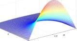
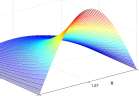
Figure 13.20: A. Graph in 3-dimensional space of u(x, t) = e 1 sinx. B. Graph of lt(x, t) = e 0M sinx.

Explore 13.4.1 For any salt concentration, u(x, t), the amount of salt in the tube at time t is / 0 u(x, t) dx. Show that for u(x, t) = e~ kt sinx, 0 < x < n, the amount, of salt in the tube at time t is 2e~ kt . In both cases, Jq u(x,t) dx is initially 2 and decreases with time; the amount of salt in the tube is decreasing and salt must be leaking out the ends.

The initial concentration of salt in the rod is required in order to compute the concentration at later times. Assume that there is a known function g such that at time t = 0 the concentration at position x is g(x). Then

u(x, 0) = g(x) 0 < x < L Initial condition. (13.24)

Finally we need some knowledge about the ends of the rod, referred to as boundary conditions. The ends may be sealed so that no salt diffuses past either end. This is expressed as

u x (0,t) = u x (L,t) = 0, 0<t, Insulated boundary conditions. (13.25)

Alternatively, we might assume the rod connects two reservoirs in which the salt concentration is constant, salt may diffuse into or out of the reservoir, but there is no flow of solvent into or out of the rod. Then there will be two concentrations, Co and Cl, such that

CHAPTER 13. TWO VARIABLE CALCULUS AND DIFFUSION

578

Explore 13.4.2 Suppose the x = 0 end of the tube is attached to a reservoir with salt concentration cq — 1 and the x = L end of the tube is sealed. What would be the boundary-conditions? What would u(x,t) be for ‘large’ values of t?

Equation 13.23 for which u(x,t) is concentration of salt also describes the temperature, u(x,t), in a rod of length L that is insulated along its sides. In this case, the initial condition g(x) would be the temperature distribution along the rod at time t — 0. The rod may also be insulated at each end and boundary condition 13.25 would apply, and this accounts for the name ‘Insulated boundary condition.’ Alternatively, one end of the rod may be exposed to, say, steam and the other end exposed to ice water, and Fixed Boundary Condition 13.26 would apply.

Explore 13.4.3 Suppose on a flat sandy beach the temperature at a depth of 2 meters is constant, equal to 20°C, and the temperature at the surface of the beach is 27 + 4 sin((27r/24)t) °C. Suppose the sand temperature varies only vertically. What equations would you like to solve if you were interested in a nest of turtle eggs buried 80 cm?

There are analytical solutions to the diffusion equation 13.23 with initial condition 13.24 with either of the boundary conditions 13.25 or 13.26. Only a few of them are simple enough for our use. We describe one example and include two examples in Exercises 13.4.5 and 13.4.10.

Example 13.4.1 Problem. Let

u(x,t) = 30*(l-e-*cos7r*:r) 0<x<2 0 < t. (13.27)

Show that

u t (x, t) — \u xx (x, t), u(x, 0) = 30 * (1 — cos7r:r), and Ux [^l !! (13.28)

7T U x [2,t) — 0.

Assuming Equations 13.28 are correct, u(x,t) would describe the temperature in a rod of length 2 that is perfectly insulated along its side, had an initial temperature of 30 * (1 — cos7r:r) at position x, and was perfectly insulated on each end. The diffusion coefficient of the material in the rod is k = 1/n 2 . Alternatively, the equations would describe the salt concentration in a tube closed at each end when the initial salt concentration at position x was 30 * (1 — cos7r:r).

Explore 13.4.4 What will be the ‘eventual’ temperature distribution (or salt concentration) in the rod (tube)?

A graph of the initial temperature distribution appears in Figure 13.21A, and graphs of the temperature at times 0, 0.5, 1, 1.5 and 2 appear in Figure 13.21B. Solution. First compute some partial derivatives.

u(x,t) = 30(1 – e~* cos nx) (13.29)

ut(x,t) = 30(0 – (e -t )(-l) cos irx) = 30e _ * cos(ttx) (13.30)

u x (x,t) = 30(0 — e~'(— sin 7ra;)(7r) = 307re * sin irx (13.31)

CHAPTER 13. TWO VARIABLE CALCULUS AND DIFFUSION

579

A

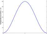
B

Temperature

Distance, x, along a rod

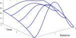
Figure 13.21: Partial graphs of Equation 13.27. A. Graph of temperature at time t — 0. B. Graphs of the temperature at times 0, 0.5, 1.0, 1.5 and 2.0. The graphs of temperature at the ends x = 0 and x = 2 are included.

From Equations 13.30 and 13.32

Ut(x, t) = 30e cos(7nc) = —^30^ e cos(7ra:) = — *u xx .

7T 7T

From Equation 13.27

From Equation 13.31,

u(x, 0) = 30 * (1 — e * cos ir * x) ^ = 30(1 — cos irx).

u x (0,t) = 30ive *sin7ra; = 0 and u x (2,t) = 30ire *sin7ra: Thus all of Equations 13.28 are satisfied.

x=2

13.4.1 Numerical solutions to the diffusion equation.

Finding analytic solutions to the diffusion equation is beyond the scope of this text. However, a numerical scheme for approximating a solution is well within reach.

Partition the tube into n intervals of length d = L/n, and partition time into intervals of length 5, as shown in Figure 13.22 for n = 5 and the space time grid shown above the tube.

Begin with Equation 13.23,

u t (x,t) = ku xx (x,t)

From Equations 9.22 and 9.24

, . u(x,t + 8) — u(x, t) . , . u(x + d, t) — 2u(x, t) + u(x — d, t) u t {x,t) = and u xx (x,t) = 2 .

d z

Using these in the previous equation leads to

u(x, t + 8) — u(x, t) . u(x + d, t) — 2u(x, t) + u(x — d, t)

(13.33)

Now we write an exact equation

v i,j+l ~~ v i,j _ ~ 2>Vij + Vi-ij

(13.34)

I I I I I I

ta = 36 j^ V 0,3 j^l,3 _^_V2,3 _|_1>3,3 _|_«4,3 _|_«5,3

t 2 = 25 + V °’ 2 +” 1 ‘ 2 + V2 ‘ 2 + V3,2 +^ 4 ‘ 2 +^ 5 ‘ 2

ti = ^ _|_”0,1 ^1,1 ^2,1 V 3 ,l _|_«4,1 _|_«5,1

^ = Q _|_WO,0 ^1,0 ^2,0 W3.0 _|_«4,0 _|_«5,0

5(x 0 ) 3(2:1) g(x 2 ) g(x 3 ) g(x 4 ) g(x 5 ) l l

I ! ! ! ! I

X 0 X\ x 2 x 3 x 4 x 5

Figure 13.22: Glass tube and grid for diffusion computation.

where Vij is an approximation to u(i * d,j * 5). Equations 13.34 can be solved as is illustrated in the next example. Using this notation in Equation 13.34 and rearranging leads to

k 5

Vij+i = Vij + k (ui-ij – 2vij + v i+hj ) where k = (13.35)

Equation 13.35 defines Vij+i (at time value j + l)in terms of Vi-ij, v^j and v i+ j, values of v at the immediately preceding time value j. See Figure 13.23. The computation is started at time j = 0 with values of v^q equal to values of the initial condition g(x) and progresses ‘upward’ in time, one layer at a time.

Example 13.4.2 Assume there is a glass tube of length L — 1 meter and of cross sectional area A = 1 cm filled with water; initially there is no salt in the tube; the left end is attached to a salt water reservoir with salt concentration = 1 and the right end is attached to a pure water reservoir. Let u(x, t) be the salt concentration in the tube at position x and time t.

Explore 13.4.5 What do you expect the ‘eventual’ salt concentration along the tube to be?

The diffusion equation is u t (x,t) = ku xx (x,t). Because initially there is no salt in the tube, g(x) = 0 for 0 < x < 1, and the reservoirs at the ends of the tube imply the fixed boundary conditions 13.26, u(0,t) = 1 and u(l,t) = 0, 0 < t.

Partition the tube into 5 equal intervals. There is in Figure 13.22 an array of points horizontally distributed with position x along the tube and distributed vertically in time t.

CHAPTER 13. TWO VARIABLE CALCULUS AND DIFFUSION

581

I I I I I I I

+ + + + + + +

u + i + + + + Vi,j+l + + +

+ + + + + + +

Figure 13.23: Geometric arrangement of the grid points of Equation 13.35. In this example,

Vij = u(i x 1/5, j x 5), i = l,5, j = !,•••. and from Equation 13.34

k 5

Vij+i = + k (vi-ij – 2vij + v i+ ij) where k = (13.36)

The boundary conditions 13.26 with u(0,t) = 1 and u(l,t) = 0 lead to

v Q j = 1 v 5 j = 0 (13.37)

The initial condition and equations 13.36 determine the v^j one horizontal layer at a time for the interior grid points, 1 < i < 5.

Begin with the initial condition, Equation 13.24:

Vi, 0 = g(xi) =0, 2 = 1,4 (13.38)

Then for the bottom layer of the grid in Figure 13.22

v 0fi = 1 and v jfi = 0 j = 1, • • •, 5.

Then compute the next layer up for t = 5:

CHAPTER 13. TWO VARIABLE CALCULUS AND DIFFUSION

582

Table 13.1: A MATLAB program that computes approximations from Equations 13.36-13.38 with k = 0.2

close all;clc;clear for j = 1:6 v(l,j)=0;

end

v(l,l)=l; for i = 2:16 v(i,l)=l; v(i,6)=0; for j = 2:5

dd=v(i-l,j-l)-2*v(i-l,j)+v(i-l,j+1); v(i,j) = v(i-l,j)+0.2*dd;

end

end

u=flipud(v)

In a similar way as many layers as necessary can be computed. The computations for k = 0.2 are shown below. The next MATLAB program produces the computations that appear in Table 13.1.

Remember that k diffusion constant, k.

kS d 2

incorporates the time step, S, and dimension step, d, as well as the

These computations may be visualized as salt (gray color) migrating to the right in a tube as illustrated in the graphic. M

The data are printed as we have been discussing, with t increasing upward. This is accomplished by the peculiar last command u = f lipud(v) . You may prefer replacing this with the command u = v for some applications.

CHAPTER 13. TWO VARIABLE CALCULUS AND DIFFUSION

583

The notation v(i, j) is consistent with our previous discussion, but some technologies, particularly programmable hand calculators, may not have the two dimensional arrays or may be limited with the size of such arrays. The following equivalent program demands less storage and produces the same data, but not with the same vertical orientation.

close all;clc;clear for j = 1:6 oldv(j)=0;

end

oldv(l)=l; oldv

for i = 2:16 oldv(l)=l; oldv(6)=0; for j = 2:5

dd=oldv(j-l)-2*oldv(j)+oldv(j+l);

newv(j) = oldv(j)+0.2*dd;

end newv

oldv=newv;

end

k 8

There is a severe constraint on k = m order that Equations 13.35 yield values of Vij that reasonably approximate the target function u(x,t). We must have

? k 5 1 .„ „

k = < (13.39)

The consequence of k > 1/2 is illustrated in Exercise 13.4.1b, where k = 0.6. In Example 13.4.2 the tube partition is d = 0.2 meters. If one wanted a smaller partition in order to more accurately approximate the salt concentration, say d = 0.01, one centimeter or l/20th of the space step of the example, then the time step 8 would have to be l/400th of the first time dimension. It would take 400 iterations of the resulting equations in order to move one of the original time steps. There is an interesting alternate procedure that is not so constrained that will be found in numerical analysis books.

Exercises for Section 13.4, The diffusion equation.

Exercise 13.4.1 1. Use MATLAB or similar technology to run a program similar to or the same as that of Table 13.1, run it, and confirm the computations shown in Table 13.1.

2. The program is written for k = 0.2. Alter the program so that k = 0.6 and run it. Do the computed approximations match what you think will be the salt concentrations?

3. The program is written for k = 0.2. Alter the program so that k — 0.1 and run it. Is the last temperature distribution in the rod at equilibrium?

4. Retain k — 0.1 and change i = 2:17 to i = 2:100 . Now is the last temperature distribution close to equilibrium?

CHAPTER 13. TWO VARIABLE CALCULUS AND DIFFUSION

584

Exercise 13.4.2 a. Use MATLAB or similar technology to run a program similar to or the same as that of Table 13.1; alter it to accommodate 10 intervals in [0,1] for x. Retain k = 0.2. Run the program and observe the result.

b. The x-interval d — 0.1, is now one-half of the previous value of 0.2, and

l_k5

Assume that the conductance coefficient, k, has not changed. How must the time increment, 5, change in order that k and k be the same as before and d be one-half of its previous value?

c. Run your program. What values in the new data most closely correspond to values in Table 13.1.

Exercise 13.4.3 Solve Equations 13.36, 13.37, and 13.38 using an Excel spread sheet.

Exercise 13.4.4 A number of diffusion simulator programs can be found with Google, “diffusion simulator”. Most seemed to be blocked to public access, however, and most will require your computer to be able to run Java Applets. Try to find access to a diffusion simulator and run some experiments on it.

Exercise 13.4.5 a. Show that

u(x, t) = 20 e~* sin ttx, 0<x<1, 0<t (13.40)

solves

u t (x, t) — — j u xx (x, t), u(x, 0) = 20 sinvra;, and u(0, t) — u(l, t) — 0 (13.41)

7T

b. Describe a physical problem for which this is a solution.

c. What is the ‘eventual’ value of u(x,t) (what is lim^^ u(x, £))?

d. At what time, t, will the maximum value of u(x, t) for 0 < x < 1 be 20?

Exercise 13.4.6 In Example 13.4.2, what is

lim u(x, t) ?

Alternatively, what is

lim vu ?

The columns of Table 13.1 may suggest an answer.

Exercise 13.4.7 a. How should the MATLAB program in Table 13.1 be modified if initially the salt concentration in the tube were 0.5?

b. If initially the salt concentration at position x in the tube is x?

CHAPTER 13. TWO VARIABLE CALCULUS AND DIFFUSION

585

Exercise 13.4.8 For the insulated ends boundary condition 13.26

u x (0,t) — 0 and u x (L,t) — 0, you might approximate these partial derivatives with the difference quotients

, , u(Q + d,t)-u(Q,t) , . « u(L,t) -u(L – d.t)

«x(0,t) = – — A — and Ux (L,t) = -L-L^ -i l2.

a a

Then-u x (0,t) = 0 and u x (L, t) = 0 would lead to

■u(0, i) = u(0 + d, t) and u(L,t) — u(L — d,t). Suppose the initial condition is

u(x, 0) = x

a. Modify the MATLAB program in Table 13.1 (better, modify the MATLAB program of Exercise 13.4.2) to use this boundary condition and initial condition.

b. Run the program and report the result.

c. What do you expect

lim u(x, t) to be?

Exercise 13.4.9 a. For any g(x), how much salt is in the rod (of length 1 meter and cross section 1cm 2 ) at time t — 07 Consider some special cases such as g(x) = lg/cm 3 and g(x) = x g/cm 3 . Then for general g, think, approximately how much salt is in the first 10 cm of the rod, the second 10 cm of the rod, • • •, the last 10 cm of the rod, and add those quantities.

b. For the insulated end boundary condition 13.26 and any initial condition g(x) and rod length L what is

lim u(x, t) ?

Exercise 13.4.10 Suppose there is an infinitely long tube containing water lying along the X-axis from —oo to oo and at time t = 0 a bolus injection of one gram of salt is made at the origin. Let u(x,t) be the concentration of salt at position x in the tube at time t.

Considering t = 0 is a bit stressful. The bolus injection of one gm at the origin causes the concentration at x = 0 and t = 0 to be rather large; u(0, 0) = oo; but u(x, 0) = 0 for x ^ 0.

Moving on, we assume that for t > 0

u t (x,t) = ku xx (x,t) (13.42) where the diffusion coefficient, k, describes the rate at which salt diffuses in water, a. Show that

u(x, t) = -jL= e 2 /(4fci) ( 13 43)

is a solution to Equation 13.42.

b. Suppose k = 1/4. Sketch the graphs of u(x, 1), 4), and u(x,S).

CHAPTER 13. TWO VARIABLE CALCULUS AND DIFFUSION

586

c. Suppose k — 1/4. Sketch the graphs of u(x, 1), u(x, 1/2), and u(x, 1/4).

d. Estimate the areas under the previous curves. For any time, to, what do you expect to be the area under the curve of u(x, t 0 ), oo < x < oo.

Exercise 13.4.11 Diffusion in two dimensions is similar to that in one dimension. The two-dimensional diffusion equation is

1. Suppose a square thin copper plate is embedded in perfect thermal insulation with only one edge exposed. Initially the plate is at 0°C. Then 100°C steam passes over the exposed edge. Describe how you might approximate the temperature distribution within the plate as time progresses.

2. A single instance of a highly contagious influenza occurs at the center of a square city and diffuses through the uniformly distributed population according to Equation 13.44, with u(x,y,t) being the fraction of the population at location (x,y) that is infected at time t. Describe how you may approximate the progress of the disease as a function of time.

Chapter A

Summation Notation and Mathematical Induction

A.l Summation Notation.

We use the symbol,

, called an ellipsis. Consider the sum

gx2

1\ 2 /2\ 2

to) + y +

+

10

+

10\ 2

10/

The ellipsis,

replaces some of the terms. In this particular instance, • • • replaces

3\ 2 /4\ 2

10) + y +

10

+

6

To

+

7- 1 10,

8V 10/

The excitement of writing these additional terms is rather limited, and most students readily accept this abbreviation 1 . It is particularly useful in writing sums with 1000 or more terms. On occasions, one sees something like

10

+

2 \ 2

To) +

+

hi

10

+ ••■ +

10\ 2 10 J

x

1

To

The term (J^J is a generic formula for the kth term in the sum. The generic term is useful, and it is important to be able to recognize a pattern for the terms of the sum. When k — 1 is substituted into the generic formula (^j^J we get (^j^j which is the first term of the sum. Similarly, substitution of k = 2 yields the second term, and substitution of k — 10 yields the 10th term.

1 This is easily grasped, as illustrated by the title of a children’s book, “One, Two, Skip a Few, Ninety-nine, One Hundred”.

CHAPTER A. SUMMATION NOTATION AND MATHEMATICAL INDUCTION

588

Some sums and generic terms are illustrated below.

V7 + v / 8 + V9

10

y/7 + V8 + V9 + V^O + Vn l 2 + 3 2 + 5 2 + 7 2 + 9 2 + ll 2

5^4^3^2^1

– + — + — + — + — + 1 2 ~ 2.2 ~ 2.4 ~ 2.6 ~ 2.8 ~ 3

(2k-if

1

6 -A;

li

fc=7 5

fc=i

ELi(2*-i) a

5 1

E

fc=i

6

6 — A;

i y 1

1.8 + k x 0.2 ^ 1.8 + Jfe x 0.2

sin(|)+ sin(2|)+ sin(3f)+ sin(4|)+ sin(5|) sin(A;f) ^ sin(A;-)

k=i

There is a compact notation that focuses attention on the generic term:

10

E

fc=i

-) x -10/ 10

J2 is the Greek letter, capital sigma, to which the Latin letter S corresponds, and symbolizes sum. The entire symbol is read “The sum from k equal to 1 to 10 of times It may also be read

as “The sum from k equal to 1 to k equal to 10 of (J^j times ^” and might be written

10

E

k=i

10

10

or

k=i

10

10

The second form is ambiguous, but both are the same because of the distributive property of the number system. The sums

10

E

k=l

10

1

To

and

k=10 ( j.

E ” !

k=i

10

+

10

are ambiguous and are not equal.

10

E

k=i

k_Y JL_ 10/ + 10

E (k

k=i

10

+

10

Typesetters find the £ notation preferable as it is much more compact. In fact, after you use it a while, you will likely find that you can more quickly grasp the meaning of the sum with the shorter notation.

It will help you to use algebra like

k=i

10

10

10 / k

E

k=i

10

x

CHAPTER A. SUMMATION NOTATION AND MATHEMATICAL INDUCTION

589

This is use of the distributive property, and can be seen from long notation with which you are familiar:

1 \ 2 1

— x — 10/ 10

10

E

k=l

2 V

— x — 10/ 10

9

1

1_\ 2 /2_2 10/ + I10

+ ••• +

10/ 10

9 x2

10

10

E

k=l

X

10

_fc 10 /

10\ 2 1

— x — 10/ 10

ioy

10/

10

1

To

A.2 Mathematical Induction.

Mathematical Induction is a powerful way of thinking that allows one to prove an infinite number of statements with a finite set of sentences. That is a pretty good trade.

We use the method of Mathematical Induction to show that Equation 9.4,

o o o o l9 n(n + l)(2n + l)

l 2 + 2 2 + 3 2 + ■■■+ n 2 = Y< k = ~

k=l

6

is valid for all integers n. The method extends to many equations and other settings. To show its use in other settings we describe the problem of the “Tower of Hanoi” and its solution.

Example A.2.1 Demonstration of the validity of

099 9 n(n + 1) (2n + 1)

l 2 + 2 2 + 3 2 + • • • + n 2 =

6

For every positive integer, n, let S n be the statement

999 9 n(n + 1) (2n + 1)

l 2 + 2 2 + 3 2 + • • • + n 2 =

Then Si is the statement,

2 = 1 (1 + 1) (2 • 1 + 1) = 6 6 6

6

1, statement Si is true,

CHAPTER A. SUMMATION NOTATION AND MATHEMATICAL INDUCTION

590

and the Induction Hypothesis 1 is satisfied.

Suppose n is a positive integer and S n is true. Then

999 9 n(n + 1) (2n + 1)

l 2 + 2 2 + 3 2 + — + n 2 = v M ^

6

V + 2 2 + r + • • • + n 2 + (n + 1)

2 _ n(n+l)(2n + l) +(n + 1)2

6

n(n + 1) (2n + 1) + 6(n + l) 2 6

(n + l)(n(2n + l) + 6(n + l)) 6^

(n + l)(2n 2 + 7n + 6)) 6

(n + l)(n + 2)(2n + 3) 6

9 9 9 9 . n9 (n + l)((n+l) + l)(2(n+l) + l)

l 2 + 2 2 + 3 2 + — + n 2 + (n + l 2 = v AV ; A v ; ;

6

The last equation is SVt+i- On the assumption that S n is true, we have shown that S n+ i is true, and the Induction Hypothesis 2 is satisfied. Therefore, every statement in Si, 5*2, 5*3, • • • is true. End of Proof, h

Example A.2.2 .

There is a puzzle in which there is a board with three vertical spikes. On one of the spikes there is a stack of round discs no two of which are of the same size, and no disc of one size is on top of a disc of a smaller size. See Figure A.l

Figure A.l: A picture of the puzzle, The Tower of Hanoi, copied from http://en.wikipedia.org/wiki/Tower_of_Hanoi, figure posted by iEvar Arnfjoro Bjarmason.

The objective of the puzzle is to move the entire stack to another rod, obeying the following rules:

• Only one disk may be moved at a time.

• Each move consists of taking the upper disk from one of the spikes and placing it on another spike (there may be disks already on that spike).

CHAPTER A. SUMMATION NOTATION AND MATHEMATICAL INDUCTION

591

• No disk may be placed on top of a smaller disk.

The question is “Can the puzzle be solved for all numbers of discs on the first spike?” Consider some early cases.

Case of one disc. If there is only one disc, easy. Move that disc to another spike. Case of two discs. Still pretty easy. Move the top disc to another spike; move the bottom disc to the remaining spike; put the top disc on top of the bottom disc. Case of three discs. Not too hard, and we leave this case for you to do. Induction. For each positive integer, n, let S n be the statement

S n : The puzzle with n discs can be solved.

Our goal is to prove that all of the statements, Si, S2, ■ ■ ■ are true. We have just seen that the puzzle with one disc can be solved. Therefore, Si is true and Induction Hypothesis 1 is satisfied.

We do not have to prove it, but we also showed that S 2 is true. Induction Hypothesis 2. Suppose n is a positive integer, and S n is true. Consider a puzzle with n + 1 discs.

• S n is true, so the puzzle with n discs can be solved. Use those steps to move the top n discs to another spike.

• Move the bottom disc to the empty spike.

• Move the top n discs from the spike on which you put them onto the spike that has the bottom disc.

The puzzle with n + 1 discs has been solved, so S„ + i is true. By the induction hypothesis, all of Si, S2, • ■ • are true.

Explore A.2.1 The puzzle with one disc was solved with one step. The puzzle with two discs was solved with three steps. Compute the number of steps to solve the puzzles with 3, 4, and 5 discs, and guess a formula for the number of steps to solve the n-disc puzzle. Prove by induction that your formula is correct.