
2.6: Continuity


- Last updated
- Jun 6, 2019
- Save as PDF
( \newcommand{\kernel}{\mathrm{null}\,}\)
Summary: For a function to be continuous at a point, it must be defined at that point, its limit must exist at the point, and the value of the function at that point must equal the value of the limit at that point. Discontinuities may be classified as removable, jump, or infinite. A function is continuous over an open interval if it is continuous at every point in the interval. It is continuous over a closed interval if it is continuous at every point in its interior and is continuous at its endpoints.
Many functions have the property that their graphs can be traced with a pencil without lifting the pencil from the page. Such functions are called continuous. Other functions have points at which a break in the graph occurs, but satisfy this property over intervals contained in their domains. They are continuous on these intervals and are said to have a discontinuity at a point where a break occurs.
We begin our investigation of continuity by exploring what it means for a function to have continuity at a point. Intuitively, a function is continuous at a particular point if there is no break in its graph at that point.
Continuity at a Point
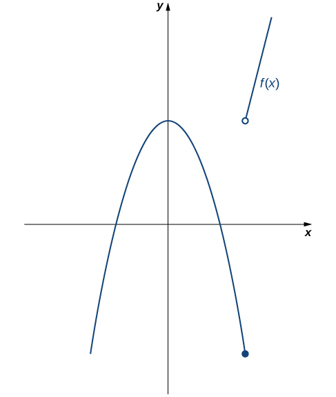
Before we look at a formal definition of what it means for a function to be continuous at a point, let’s consider various functions that fail to meet our intuitive notion of what it means to be continuous at a point. We then create a list of conditions that prevent such failures.
Our first function of interest is shown in Figure. We see that the graph of
i.
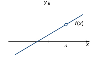
Figure
However, as we see in Figure, this condition alone is insufficient to guarantee continuity at the point a. Although
ii.
ii.
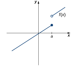
Figure
However, as we see in Figure, these two conditions by themselves do not guarantee continuity at a point. The function in this figure satisfies both of our first two conditions, but is still not continuous at a. We must add a third condition to our list:
iii.
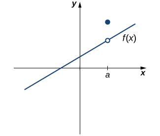
Figure
Now we put our list of conditions together and form a definition of continuity at a point.
Definition
A function
A function is discontinuous at a point a if it fails to be continuous at a.
The following procedure can be used to analyze the continuity of a function at a point using this definition.
Problem-Solving Strategy: Determining Continuity at a Point
- Check to see if
- Compute
- Compare
The next three examples demonstrate how to apply this definition to determine whether a function is continuous at a given point. These examples illustrate situations in which each of the conditions for continuity in the definition succeed or fail.
Example
Using the definition, determine whether the function
Solution
Let’s begin by trying to calculate
Figure
Example
Using the definition, determine whether the function
Solution
Let’s begin by trying to calculate
Thus,
and
Therefore,
Figure
Example
Using the definition, determine whether the function
Solution
First, observe that
Next,
Last, compare
Since all three of the conditions in the definition of continuity are satisfied,
Exercise
Using the definition, determine whether the function
- Hint
-
Check each condition of the definition.
- Answer
-
f is not continuous at 1 because
By applying the definition of continuity and previously established theorems concerning the evaluation of limits, we can state the following theorem.
Continuity of Polynomials and Rational Functions
Polynomials and rational functions are continuous at every point in their domains.
Proof
Previously, we showed that if
□
We now apply Note to determine the points at which a given rational function is continuous.
Example
For what values of x is
Solution
The rational function
Exercise
For what values of x is
- Hint
-
Use Note
- Answer
-
Types of Discontinuities
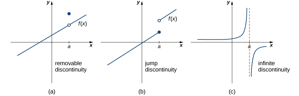
As we have seen in Example and Example, discontinuities take on several different appearances. We classify the types of discontinuities we have seen thus far as removable discontinuities, infinite discontinuities, or jump discontinuities. Intuitively, a removable discontinuity is a discontinuity for which there is a hole in the graph, a jump discontinuity is a noninfinite discontinuity for which the sections of the function do not meet up, and an infinite discontinuity is a discontinuity located at a vertical asymptote. Figure illustrates the differences in these types of discontinuities. Although these terms provide a handy way of describing three common types of discontinuities, keep in mind that not all discontinuities fit neatly into these categories.
Figure
These three discontinuities are formally defined as follows:
Definition
If
1.
2.
3.
Example
In Example, we showed that
Solution
To classify the discontinuity at 2 we must evaluate
=
=
=
Since f is discontinuous at 2 and
Example
In Example, we showed that
Solution
Earlier, we showed that f is discontinuous at 3 because
Example
Determine whether
Solution
The function value
Exercise
For
- Hint
-
Follow the steps in Note. If the function is discontinuous at 1, look at
- Answer
-
Discontinuous at 1; removable
Continuity over an Interval
Now that we have explored the concept of continuity at a point, we extend that idea to continuity over an interval. As we develop this idea for different types of intervals, it may be useful to keep in mind the intuitive idea that a function is continuous over an interval if we can use a pencil to trace the function between any two points in the interval without lifting the pencil from the paper. In preparation for defining continuity on an interval, we begin by looking at the definition of what it means for a function to be continuous from the right at a point and continuous from the left at a point.
Continuity from the Right and from the Left
A function
A function
A function is continuous over an open interval if it is continuous at every point in the interval. A function
Requiring that
Example
State the interval(s) over which the function
Solution
Since
Example
State the interval(s) over which the function
Solution
From the limit laws, we know that
Exercise
State the interval(s) over which the function
- Hint
-
Use Example as a guide for solving.
- Answer
-
[−3,+∞)
The Note allows us to expand our ability to compute limits. In particular, this theorem ultimately allows us to demonstrate that trigonometric functions are continuous over their domains.
Composite Function Theorem
If
Before we move on to Example, recall that earlier, in the section on limit laws, we showed
Example
Evaluate
Solution
The given function is a composite of
Exercise
Evaluate
- Hint
-
- Answer
-
0
The proof of the next theorem uses the composite function theorem as well as the continuity of
Continuity of Trigonometric Functions
Trigonometric functions are continuous over their entire domains.
Proof
We begin by demonstrating that
=
=
=
=
The proof that
□
As you can see, the composite function theorem is invaluable in demonstrating the continuity of trigonometric functions. As we continue our study of calculus, we revisit this theorem many times.
The Intermediate Value Theorem
Functions that are continuous over intervals of the form
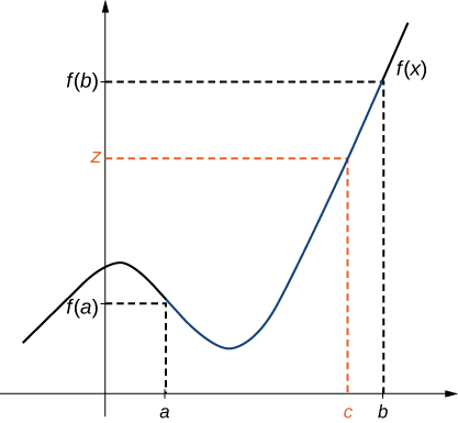
The Intermediate Value Theorem
Let f be continuous over a closed, bounded interval
Figure
Example
Show that
Solution
Since
and
Using the Intermediate Value Theorem, we can see that there must be a real number c in
Example
If
Solution
No. The Intermediate Value Theorem only allows us to conclude that we can find a value between
Example
For
Solution
No. The function is not continuous over
Exercise
Show that
- Hint
-
Find
Answer
-
Key Concepts
- For a function to be continuous at a point, it must be defined at that point, its limit must exist at the point, and the value of the function at that point must equal the value of the limit at that point.
- Discontinuities may be classified as removable, jump, or infinite.
- A function is continuous over an open interval if it is continuous at every point in the interval. It is continuous over a closed interval if it is continuous at every point in its interior and is continuous at its endpoints.
- The composite function theorem states: If
- The Intermediate Value Theorem guarantees that if a function is continuous over a closed interval, then the function takes on every value between the values at its endpoints.
Glossary
- continuity at a point
- A function
- continuity from the left
- A function is continuous from the left at b if
- continuity from the right
- A function is continuous from the right at a if
- continuity over an interval
- a function that can be traced with a pencil without lifting the pencil; a function is continuous over an open interval if it is continuous at every point in the interval; a function
- discontinuity at a point
- A function is discontinuous at a point or has a discontinuity at a point if it is not continuous at the point
- infinite discontinuity
- An infinite discontinuity occurs at a point a if
- Intermediate Value Theorem
- Let f be continuous over a closed bounded interval [
- jump discontinuity
- A jump discontinuity occurs at a point a if
- removable discontinuity
- A removable discontinuity occurs at a point a if
Contributors
Gilbert Strang (MIT) and Edwin “Jed” Herman (Harvey Mudd) with many contributing authors. This content by OpenStax is licensed with a CC-BY-SA-NC 4.0 license. Download for free at http://cnx.org.