
12.2: The Calculus of Vector-Valued Functions


- Last updated
- Jan 6, 2020
- Save as PDF
( \newcommand{\kernel}{\mathrm{null}\,}\)
To study the calculus of vector-valued functions, we follow a similar path to the one we took in studying real-valued functions. First, we define the derivative, then we examine applications of the derivative, then we move on to defining integrals. However, we will find some interesting new ideas along the way as a result of the vector nature of these functions and the properties of space curves.
Derivatives of Vector-Valued Functions
Now that we have seen what a vector-valued function is and how to take its limit, the next step is to learn how to differentiate a vector-valued function. The definition of the derivative of a vector-valued function is nearly identical to the definition of a real-valued function of one variable. However, because the range of a vector-valued function consists of vectors, the same is true for the range of the derivative of a vector-valued function.
Definition: Derivative of Vector-Valued Functions
The derivative of a vector-valued function ⇀r(t) is
⇀r′(t)=limΔt→0⇀r(t+Δt)−⇀r(t)Δt
provided the limit exists. If ⇀r′(t) exists, then ⇀r(t) is differentiable at t. If ⇀r′(t) exists for all t in an open interval (a,b) then ⇀r(t) is differentiable over the interval (a,b). For the function to be differentiable over the closed interval [a,b], the following two limits must exist as well:
⇀r′(a)=limΔt→0+⇀r(a+Δt)−⇀r(a)Δt
and
⇀r′(b)=limΔt→0−⇀r(b+Δt)−⇀r(b)Δt
Graphical Interpretation of the Derivative: Recall that the derivative of a real-valued function can be interpreted as the slope of a tangent line or the instantaneous rate of change of the function. The derivative of a vector-valued function can be understood to be an instantaneous rate of change as well; for example, when the function represents the position of an object at a given point in time, the derivative represents its velocity at that same point in time.
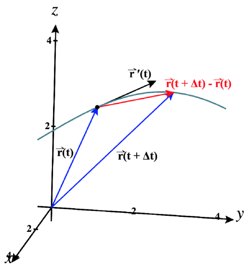
To understand what this derivative represents geometrically, it helps to consider the diagram shown in Figure 12.2.1. For the purposes of this illustration, consider ⇀r(t) to the represent position of an object.
We see vectors ⇀r(t) and ⇀r(t+Δt), where Δt is a small change in time producing a second vector that is farther along in the direction of motion.
The difference of these two vectors gives us the displacement vector, ⇀r(t+Δt)−⇀r(t), shown here in red.
As Δt→0, ⇀r(t+Δt) will approach ⇀r(t), and the displacement vector ⇀r(t+Δt)−⇀r(t) will become closer and closer to being tangent to the curve at the terminal point of ⇀r(t).
Although the length of the displacement vector is approaching 0, we are actually taking the limit not of the displacement vector itself, but of the average velocity over the time Δt, found by dividing the displacement vector by the scalar Δt.
Average Velocity=⇀r(t+Δt)−⇀r(t)Δt
Since Δt is also approaching 0, dividing by it will tend to lengthen the average velocity vector (as long as Δt<1).
The limit gives us the vector ⇀r′(t), the velocity of the motion along the curve, which is tangent to the curve at this point.
We now demonstrate taking the derivative of a vector-valued function.
Example 12.2.1: Finding the Derivative of a Vector-Valued Function
Use the definition to calculate the derivative of the function
⇀r(t)=(3t+4)ˆi+(t2−4t+3)ˆj.
Solution
Let’s use Equation ???:
\begin{align*} \vecs{r}′(t) &= \lim \limits_{\Delta t \to 0} \dfrac{\vecs{r}(t+Δt)− \vecs{r} (t)}{Δt} \\[5pt] &= \lim \limits_{\Delta t \to 0} \dfrac{[(3(t+Δt)+4)\,\hat{\mathbf{i}}+((t+Δt)^2−4(t+Δt)+3)\,\hat{\mathbf{j}}]−[(3t+4) \,\hat{\mathbf{i}}+(t^2−4t+3) \,\hat{\mathbf{j}}]}{Δt} \\[5pt] &= \lim \limits_{\Delta t \to 0} \dfrac{(3t+3Δt+4)\,\hat{\mathbf{i}}−(3t+4) \,\hat{\mathbf{i}}+(t^2+2tΔt+(Δt)^2−4t−4Δt+3) \,\hat{\mathbf{j}}−(t^2−4t+3)\,\hat{\mathbf{j}}}{Δt} \\[5pt] &= \lim \limits_{\Delta t \to 0} \dfrac{(3Δt)\,\hat{\mathbf{i}}+(2tΔt+(Δt)^2−4Δt)\,\hat{\mathbf{j}}}{Δt} \\[5pt] &= \lim \limits_{\Delta t \to 0} (3 \,\hat{\mathbf{i}}+(2t+Δt−4)\,\hat{\mathbf{j}}) \\[5pt] &=3 \,\hat{\mathbf{i}}+(2t−4) \,\hat{\mathbf{j}} \end{align*}
Exercise \PageIndex{1}
Use the definition to calculate the derivative of the function \vecs{r}(t)=(2t^2+3) \,\hat{\mathbf{i}}+(5t−6) \,\hat{\mathbf{j}}.
- Hint
-
Use Equation \ref{eq1}.
- Answer
-
\vecs{r}′(t)=4t \,\hat{\mathbf{i}}+5 \,\hat{\mathbf{j}} \nonumber
Notice that in the calculations in Example \PageIndex{1}, we could also obtain the answer by first calculating the derivative of each component function, then putting these derivatives back into the vector-valued function. This is always true for calculating the derivative of a vector-valued function, whether it is in two or three dimensions. We state this in the following theorem. The proof of this theorem follows directly from the definitions of the limit of a vector-valued function and the derivative of a vector-valued function.
Theorem \PageIndex{1}: Differentiation of Vector-Valued Functions
Let f, g, and h be differentiable functions of t.
- If \vecs{r}(t)=f(t) \,\hat{\mathbf{i}}+g(t) \,\hat{\mathbf{j}} then \vecs{r}′(t)=f′(t) \,\hat{\mathbf{i}}+g′(t) \,\hat{\mathbf{j}}.
- If \vecs{r}(t)=f(t) \,\hat{\mathbf{i}}+g(t) \,\hat{\mathbf{j}} + h(t) \,\hat{\mathbf{k}} then \vecs{r}′(t)=f′(t) \,\hat{\mathbf{i}}+g′(t) \,\hat{\mathbf{j}} + h′(t) \,\hat{\mathbf{k}}.
Example \PageIndex{2}: Calculating the Derivative of Vector-Valued Functions
Use Theorem \PageIndex{1} to calculate the derivative of each of the following functions.
- \vecs{r}(t)=(6t+8) \,\hat{\mathbf{i}}+(4t^2+2t−3) \,\hat{\mathbf{j}}
- \vecs{r}(t)=3 \cos t \,\hat{\mathbf{i}}+4 \sin t \,\hat{\mathbf{j}}
- \vecs{r}(t)=e^t \sin t \,\hat{\mathbf{i}}+e^t \cos t \,\hat{\mathbf{j}}−e^{2t} \,\hat{\mathbf{k}}
Solution
We use Theorem \PageIndex{1} and what we know about differentiating functions of one variable.
- The first component of \vecs r(t)=(6t+8) \,\hat{\mathbf{i}}+(4t^2+2t−3) \,\hat{\mathbf{j}} \nonumber is f(t)=6t+8. The second component is g(t)=4t^2+2t−3. We have f′(t)=6 and g′(t)=8t+2, so Theorem \PageIndex{1} gives \vecs r′(t)=6 \,\hat{\mathbf{i}}+(8t+2)\,\hat{\mathbf{j}} \nonumber
- The first component is f(t)=3 \cos t and the second component is g(t)=4 \sin t. We have f′(t)=−3 \sin t and g′(t)=4 \cos t, so we obtain \vecs r′(t)=−3 \sin t \,\hat{\mathbf{i}}+4 \cos t \,\hat{\mathbf{j}} \nonumber
- The first component of \vecs r(t)=e^t \sin t \,\hat{\mathbf{i}}+e^t \cos t \,\hat{\mathbf{j}}−e^{2t} \,\hat{\mathbf{k}} is f(t)=e^t \sin t, the second component is g(t)=e^t \cos t, and the third component is h(t)=−e^{2t}. We have f′(t)=e^t(\sin t+\cos t), g′(t)=e^t (\cos t−\sin t), and h′(t)=−2e^{2t}, so the theorem gives \vecs r′(t)=e^t(\sin t+\cos t)\,\hat{\mathbf{i}}+e^t(\cos t−\sin t)\,\hat{\mathbf{j}}−2e^{2t} \,\hat{\mathbf{k}} \nonumber
Exercise \PageIndex{2}
Calculate the derivative of the function
\vecs{r}(t)=(t \ln t)\,\hat{\mathbf{i}}+(5e^t) \,\hat{\mathbf{j}}+(\cos t−\sin t) \,\hat{\mathbf{k}}. \nonumber
- Hint
-
Identify the component functions and use Theorem \PageIndex{1}.
- Answer
-
\vecs{r}′(t)=(1+ \ln t) \,\hat{\mathbf{i}}+5e^t \,\hat{\mathbf{j}}−(\sin t+\cos t)\,\hat{\mathbf{k}} \nonumber
Describing Motion with Vector-Valued Functions
As has been mentioned already in this section, vector-valued functions are often used to describe motion in the plane or in space. Now that we understand the derivative of a vector-valued function, let's make the relationships clear.
First, since the components of a vector-valued function represent the coordinates of a point on the corresponding curve, it may help to write
\vecs r(t) = x(t) \,\,\hat{\mathbf{i}} + y(t) \,\,\hat{\mathbf{j}} + z(t) \, \,\hat{\mathbf{k}}
This approach has already been used in Section 12.1.
Now we can define how to calculate the velocity, speed, acceleration, and jerk of the object's motion.
Definition: Velocity, speed, Acceleration, and Jerk
Let \vecs r(t) be a twice-differentiable vector-valued function of the parameter t that represents the position of an object as a function of time.
The velocity vector \vecs v(t) of the object is given by
\text{Velocity}\,=\vecs v(t)=\vecs r′(t). \label{Eq1}
The speed is defined to be
\text{Speed}\,=‖\vecs v(t)‖=‖\vecs r′(t)‖=\dfrac{ds}{\,dt}. \label{Eq2}
The acceleration vector \vecs a(t) is defined to be
\text{Acceleration}\,=\vecs a(t)=\vecs v′(t)=\vecs r″(t). \label{Eq3}
If \vecs r(t) has a third derivative, we can also define the jerk vector \vecd{\text{jerk}}(t) to be
\text{Jerk}\,=\vecd{\text{jerk}}(t) = \vecs a'(t)=\vecs r\,'''(t). \label{Eq4}
Now let's see how this looks in the context of a particular position function.
Example \PageIndex{3}: Finding velocity, speed, acceleration, and jerk
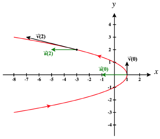
Consider the position function, \vecs r(t) = (1 - t^2) \, \hat{\mathbf{i}} + t \, \hat{\mathbf{j}}, \, \text{where time is in seconds}\nonumber
a. Determine the velocity, speed, acceleration, and jerk as functions of time for this position function.
b. Evaluate each of these functions, including the position function, at times t = 0 sec and t = 2 sec.
c. Sketch a graph of this position function and draw in each of the non-zero vectors from part b on the graph of \vecs r, starting at the location of the object on the curve at the corresponding time.
Solution
a. Since \vecs r(t) = (1 - t^2) \, \hat{\mathbf{i}} + t \, \hat{\mathbf{j}}, we have
\begin{align*} \vecs v(t) &= \vecs r\,'(t) = -2t \, \hat{\mathbf{i}} + 1 \, \hat{\mathbf{j}},\\[5pt] \text{speed}(t) &= \|\vecs v(t) \| = \sqrt{(-2t)^2 +(1)^2} = \sqrt{4t^2 + 1}, \\[5pt] \vecs a(t) &= \vecs v'(t) = -2 \, \hat{\mathbf{i}}, \\[5pt] \vecd{\text{jerk}}(t) &= \vecs 0 \end{align*}
b. Evaluating these functions at time t = 0, we get:
\begin{align*} \vecs r(0) &= (1 - 0^2) \, \hat{\mathbf{i}} + 0 \, \hat{\mathbf{j}} = \hat{\mathbf{i}} \\ \vecs v(0) &= -2(0) \, \hat{\mathbf{i}} + 1 \, \hat{\mathbf{j}} = \hat{\mathbf{j}} \\ \text{speed}(0) &= \sqrt{4(0)^2 + 1} = \sqrt{1} = 1 \, \text{unit/sec} \\ \vecs a(0) &= -2 \, \hat{\mathbf{i}}, \\ \vecd{\text{jerk}}(0) &= \vecs 0 \end{align*}
And for time t = 2, we have
\begin{align*} \vecs r(2) &= (1 - 2^2) \, \hat{\mathbf{i}} + 2 \, \hat{\mathbf{j}} = -3 \, \hat{\mathbf{i}} + 2 \, \hat{\mathbf{j}} \\ \vecs v(2) &= -2(2) \, \hat{\mathbf{i}} + 1 \, \hat{\mathbf{j}} = -4 \, \hat{\mathbf{i}} + \hat{\mathbf{j}} \\ \text{speed}(2) &= \sqrt{4(2)^2 + 1} = \sqrt{17} \, \text{units/sec} \\ \vecs a(0) &= -2 \, \hat{\mathbf{i}}, \\ \vecd{\text{jerk}}(0) &= \vecs 0 \end{align*}
c. The graph of this curve is shown below in Figure \PageIndex{2}. We then drew in and labeled the vectors \vecs v(0), \vecs a(0), \vecs v(2), and \vecs a(2).
Smooth Vector-Valued Functions
Definition: smoothness
Let \vecs{r}(t)=f(t) \,\hat{\mathbf{i}}+g(t) \,\hat{\mathbf{j}} + h(t) \,\hat{\mathbf{k}} be the parameterization of a curve that is differentiable on an open interval I.
Then \vecs r(t) is smooth on the open interval I, if
\vecs r\,'(t) \neq \vecs 0, for any value of t in the interval I.
To put this another way, \vecs r(t) is smooth on the open interval I if:
- \vecs r(t) is defined and continuous on I, and
- f', \, g' and h' are all continuous on I, that is, \vecs r\,'(t) is defined and continuous on I, and
- \vecs r\,'(t) \neq \vecs 0 for all values of t in the interval I.
The concept of smoothness is very closely connected to the application of vector-valued functions to motion. If you have ever ridden rides at an amusement park, you can probably identify some where the ride felt smooth, and others where there are moments during the ride where it was not smooth. These moments often correspond to points in the motion where the relevant parameterization is not smooth by the definition above.
To identify open intervals in the domain of \vecs r on which \vecs r is smooth, we usually identify values of t for which \vecs r is not smooth.
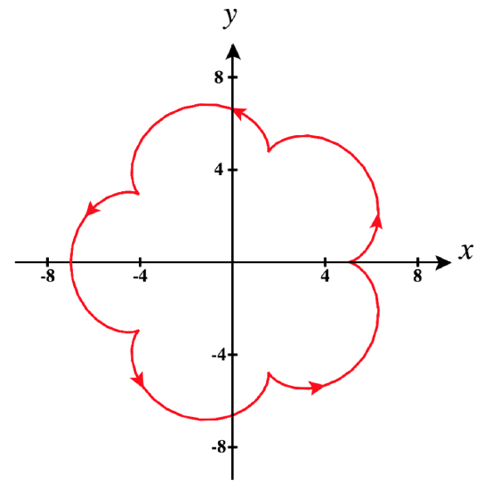
In addition to using the definition above to identify these points, it is often apparent from the graph of the vector-valued function \vecs r(t). A cusp, i.e., a sharp turning point, is a common occurrence at points where a curve is not smooth. In Figure \PageIndex{3} below, you can quickly identify points at which the parameterization fails to be smooth by locating cusps in the graph.
When we consider the motion described by \vecs r(t), there are at least two additional events that can occur at points where the parameterization fails to be smooth: a reversal of motion or a momentary pause in the motion. To summarize these events:
If a vector-valued function \vecs r(t) is not smooth at time t, we will observe that:
- There is a cusp at the associated point on the graph of \vecs r(t), or
- The motion reverses itself at the associated point, causing the motion to travel back along the same path in the opposite direction, or
- The motion actually stops and starts up again, with no visual cue, that is, where the curve appears smooth.
Let's consider a couple examples to see how this can look.
Example \PageIndex{4}: Determining open intervals on which a vector-valued function is smooth
Determine the open intervals on which each of the following vector-valued functions is smooth:
- \vecs r(t) = \left( 2t^3 - 3t^2\right) \, \,\hat{\mathbf{i}} + \left( t^2 - 2t\right) \, \,\hat{\mathbf{j}} + 2\,\,\hat{\mathbf{k}}
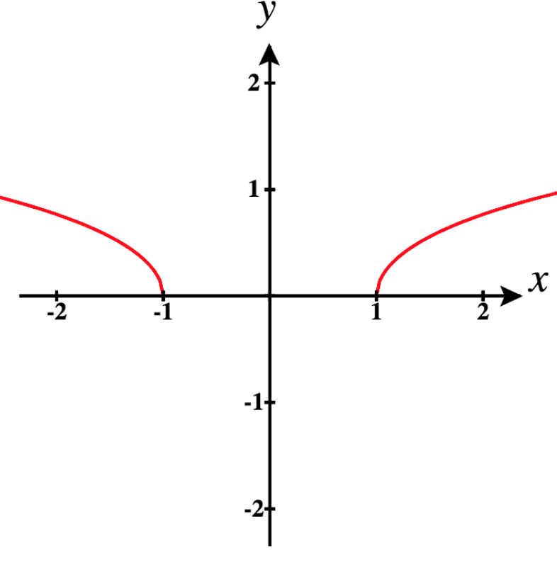
- \vecs r(t) = t^3 \, \,\hat{\mathbf{i}} + \sqrt{t^2 - 1} \,\hat{\mathbf{j}}
- \vecs r(t) = t^4 \, \,\hat{\mathbf{i}} + \ln(t^2 + 1) \,\hat{\mathbf{j}}
- \vecs r(t) = \left( 6\cos t - \cos(6t)\right) \,\hat{\mathbf{i}} + \left( 6\sin t - \sin(6t) \right) \,\hat{\mathbf{j}}, for 0 \le t \le 2\pi
Solution
a. First we need to consider the domain of \vecs r. In this case, \text{D}_{\vecs r} : (-\infty, \infty).
Then we need to find \vecs r\,'(t). Since \vecs r(t) = \left( 2t^3 - 3t^2\right) \, \,\hat{\mathbf{i}} + \left( t^2 - 2t\right) \, \,\hat{\mathbf{j}} + 2\,\,\hat{\mathbf{k}},
\vecs r\,'(t) = \left( 6t^2 - 6t\right) \, \,\hat{\mathbf{i}} + \left( 2t - 2\right) \, \,\hat{\mathbf{j}}\nonumber
Next we need to consider the domain of \vecs r\,'. Here, \text{D}_{\vecs r\,'} : (-\infty, \infty).
Finally we need to determine if there are any values of t in \text{D}_{\vecs r} where \vecs r\,'(t) = \vecs 0.
To do this, we set each component of \vecs r\,'(t) equal to 0 and solve for t.
\begin{align*} 6t^2 - 6t = 0 & \quad \text{and} \quad & 2t - 2 = 0 \\ 6t(t -1) = 0 && 2(t - 1) = 0 \\ t = 0 \quad \text{or} \quad t = 1 & & t = 1 \end{align*}
Since t = 1 makes both components of \vecs r\,' equal 0, we have \vecs r\,'(1) = \vecs 0, so we know that \vecs r is not smooth at t = 1.
Note however that \vecs r is smooth at t = 0, because although one of the components of \vecs r\,' is 0, the other one is not.
Therefore we can conclude that \vecs r is smooth on the open intervals:
(-\infty, 1) \quad \text{and} \quad (1, \infty) \nonumber
Note in the figure that there is a cusp in the curve when t = 1.
b. Next let \vecs r(t) = t^3 \, \,\hat{\mathbf{i}} + \sqrt{t^2 - 1} \,\hat{\mathbf{j}}.
The domain of \vecs r is \text{D}_{\vecs r} : (-\infty, -1] \cup [1, \infty) , since t^2 - 1 is less than 0 between -1 and 1.
Now we calculate \vecs r\,'(t). Since \vecs r(t) = t^3 \, \,\hat{\mathbf{i}} + \sqrt{t^2 - 1} \,\hat{\mathbf{j}}, we have
\vecs r\,'(t) = 3t^2 \, \,\hat{\mathbf{i}} + \frac{t}{\sqrt{t^2-1}} \, \,\hat{\mathbf{j}}\nonumber
Then, since we cannot have zero in the denominator, t = -1 and t = 1 are not in the domain of \vecs r\,'. Thus, \text{D}_{\vecs r\,'} : (-\infty, -1) \cup (1, \infty) .
Lastly we determine if there are any values of t in \text{D}_{\vecs r} where \vecs r\,'(t) = \vecs 0.
Setting each component of \vecs r\,'(t) equal to 0 and solving for t we get:
\begin{align*} 3t^2 = 0 & \quad \text{and} \quad & \frac{t}{\sqrt{t^2-1}} = 0 \\ t = 0 && t = 0 \end{align*}\nonumber
If t = 0 were in the domain of \vecs r\,', then \vecs r would not be smooth there, but since it is not in the domain, we have nothing to remove, and we can conclude that \vecs r is smooth on the entire domain of its derivative \vecs r\,', that is,
\vecs r \, \text{is smooth on the open intervals:} \quad (-\infty, -1) \quad \text{and} \quad (1, \infty).\nonumber
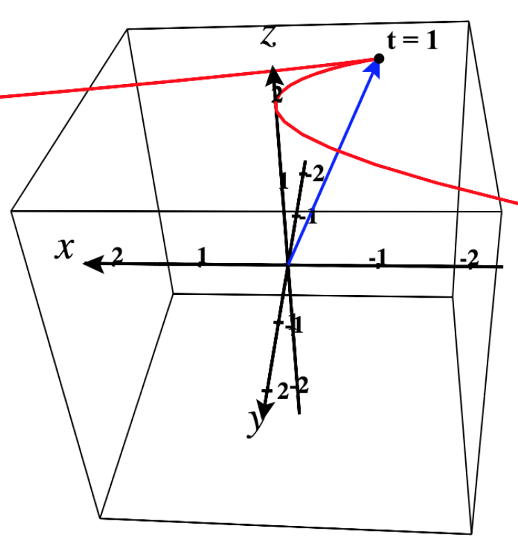
Observe the two separate smooth pieces of this function in the graph below.
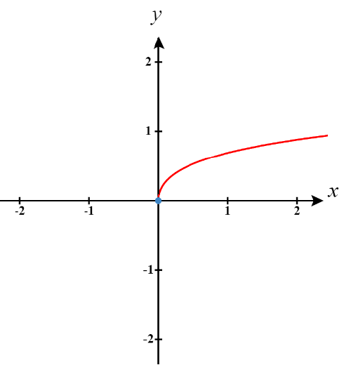
c. Now let's consider, \vecs r(t) = t^4 \, \,\hat{\mathbf{i}} + \ln(t^2 + 1) \,\hat{\mathbf{j}}.
The domain of \vecs r is \text{D}_{\vecs r} : (-\infty, \infty), since the argument of the natural log function, t^2 + 1, is always greater than 0 (In fact, it's always at least 1).
Now we calculate \vecs r\,'(t). Here
\vecs r\,'(t) = 4t^3 \, \,\hat{\mathbf{i}} + \frac{2t}{t^2+1} \, \,\hat{\mathbf{j}}\nonumber
Then, since t^2+1 cannot be 0, the domain of \vecs r\,' is also all real numbers, \text{D}_{\vecs r\,'} : (-\infty, \infty) .
Lastly we determine if there are any values of t in \text{D}_{\vecs r} where \vecs r\,'(t) = \vecs 0.
Setting each component of \vecs r\,'(t) equal to 0 and solving for t we get:
\begin{align*} 4t^3 = 0 & \quad \text{and} \quad & \frac{2t}{t^2+1} = 0 \\ t = 0 && t = 0 \nonumber \end{align*}
Note that in this example, we have \vecs r\,'(0) = \vecs 0, so \vecs r is not smooth when t = 0.
Therefore we conclude that \vecs r is smooth on the open intervals: (-\infty, 0) \quad \text{and} \quad (0, \infty) \nonumber
In this example, note that the motion reverses itself when t = 0. We can't see this very well just by looking at its graph (see Figure \PageIndex{6}). But if you evaluate \vecs r(t) for various values of t from -2 to 2, you'll see that the motion comes in towards the origin when t is negative, arrives at the origin when t=0, and then moves away from the origin as t becomes more positive.
d. Finally, let's look at a really interesting example: \vecs r(t) = \left( 6\cos t - \cos(6t)\right) \,\hat{\mathbf{i}} + \left( 6\sin t - \sin(6t) \right) \,\hat{\mathbf{j}}.\nonumber
Its graph is the epicycloid shown above in Figure \PageIndex{3}.
Again, \vecs r has no issues with its domain. We have \text{D}_{\vecs r} : (-\infty, \infty).
Calculating \vecs r\,'(t), we get:
\vecs r\,'(t) = \left( -6\sin t + 6\sin(6t)\right) \,\hat{\mathbf{i}} + \left( 6\cos t - 6\cos(6t)\right) \,\hat{\mathbf{j}}\nonumber
There are still no issues, so \text{D}_{\vecs r\,'} : (-\infty, \infty).
Now for the most interesting part! For what values of t is \vecs r\,'(t) = \vecs 0?
Setting the two components equal to 0, we get:
-6\sin t + 6\sin(6t)= 0 \quad \text{and} \quad 6\cos t - 6\cos(6t) = 0 \nonumber
This time it's not as easy to quickly solve each of these equations for all values of t that make these component functions equal to 0. But if you read carefully, you'll see that it's really not that difficult to work out.
Rewriting the first equation gives us
\sin(6t) = \sin t\label{eqSin6t}
To solve this equation, note that the periodic nature of the sine function means that its value is the same every 2\pi radians.
That is, for any integer n, we know
\sin(t+2n\pi) = \sin t \nonumber
This means that one way for Equation \ref{eqSin6t} to be true would be for us to have
t + 2n\pi = 6t\nonumber
Solving this equation for t, we have:
\qquad t = \dfrac{2n\pi}{5} \text{ for any integer }n
On the interval 0 \le t \le 2\pi, this would give us the following solutions of Equation \ref{eqSin6t}:
t = 0, \,\frac{2\pi}{5}, \,\frac{4\pi}{5}, \,\frac{6\pi}{5}, \,\frac{8\pi}{5}, \,\frac{10\pi}{5}=2\pi\nonumber
Verifying that t = \frac{2\pi}{5} is a solution, we have:
\sin\left(6\cdot \frac{2\pi}{5}\right) = \sin\left(2\pi +\frac{2\pi}{5}\right) = \sin\left(\frac{2\pi}{5}\right). \quad\checkmark \nonumber
Note that the sine value (as the y-coordinate of a point on the unit circle) is the same for reflected angles about the \(y)-axis (e.g., in the first and second quadrants). That is,
\sin(\pi - t) = \sin t \nonumber
Incorporating the periodic nature of the sine function again, we obtain
\sin\Big(\big(2n+1\big)\pi - t \Big) = \sin t \nonumber
Applying this identity to Equation \ref{eqSin6t}, yields
\sin\Big(\big(2n+1\big)\pi - t \Big) = \sin (6t) \nonumber
So, another way for Equation \ref{eqSin6t} to be true would be for us to have
(2n+1)\pi - t = 6t \nonumber
Solving this equation for t, we have:
\qquad t = \dfrac{(2n+1)\pi}{7} \text{ for any integer }n
On the interval 0 \le t \le 2\pi, this would give us the following solutions of Equation \ref{eqSin6t}:
t = \frac{\pi}{7}, \,\frac{3\pi}{7}, \,\frac{5\pi}{7}, \,\frac{7\pi}{7}=\pi, \,\frac{9\pi}{7}, \,\frac{11\pi}{7}, \,\frac{13\pi}{7} \nonumber
Verifying that t = \frac{\pi}{7} is a solution, we have:
\sin\left(6\cdot \frac{\pi}{7}\right) = \sin\left(\pi -\frac{\pi}{7}\right) = \sin\left(\frac{\pi}{7}\right). \quad\checkmark \nonumber
Next we need to solve the equation from the setting the other component of \vecs r\,'(t) to 0. That is
6\cos t - 6\cos(6t) = 0 \nonumber
Remember that not all values of t that make one of these components equal to 0 will cause \vecs r not to be smooth, but only those values of t that make both components equal to 0 at the same time. Once we solve this equation, we'll need to look for any values of t that are solutions to both of these equations.
Rewriting the equation above gives us
\cos(6t) = \cos t\label{eqCos6t}
We can solve this equation using a similar process to what was shown for Equation \ref{eqSin6t} above.
As the cosine function is periodic in the same way that sine is, we have
\cos(t+2n\pi) = \cos t
which tells us Equation \ref{eqCos6t} will be true when
t + 2n\pi = 6t\nonumber
Solving this equation for t, we have:
\qquad t = \dfrac{2n\pi}{5} \text{ for any integer }n
Note that these values for t also made the first component of \vecs r\,'(t) equal to 0! Try verifying that one of these solutions satisfies Equation \ref{eqCos6t}, as we showed for Equation \ref{eqSin6t} above.
Since the cosine values (as the x-coordinates of points on the unit circle) are the same for reflected angles about the x-axis (e.g. in the first and fourth quadrants). This is represented in the identity:
\cos(-t) = \cos(t) \nonumber
Incorporating the periodic nature of the cosine function (as we did before), we obtain
\cos(2n\pi - t) = \cos(t) \nonumber
Applying this identity to Equation \ref{eqCos6t}, yields
\cos(2n\pi - t) = \cos(6t) \nonumber
This is true when
2n\pi - t = 6t\nonumber
Solving this equation for t, we have:
\qquad t = \dfrac{2n\pi}{7} \text{ for any integer }n
Although these may at first look like the same values as we found solved Equation \ref{eqSin6t} above, they are not.
On the interval 0 \le t \le 2\pi, this would give us the following solutions of Equation \ref{eqCos6t}:
t = 0, \frac{2\pi}{7}, \,\frac{4\pi}{7}, \,\frac{6\pi}{7}, \,\frac{8\pi}{7}, \,\frac{10\pi}{7}, \,\frac{12\pi}{7}, \,\frac{14\pi}{7} = 2\pi \nonumber
Except for t = 0 and t = 2\pi that are already contained in the first set of solutions t = \dfrac{2n\pi}{5} above, this second set of solutions does not add any additional values of t that would make both components of \vecs r\,'(t) equal to 0 at the same time.
We have now determined that \vecs r\,'(t) = \vecs 0 and therefore \vecs r is not smooth when t = \dfrac{2n\pi}{5} \text{ for any integer }n.
Removing these values from the interval 0 \le t \le 2\pi, we can say that \vecs r is smooth on the open intervals:
\left(0, \,\frac{2\pi}{5}\right), \; \left(\frac{2\pi}{5} , \, \frac{4\pi}{5} \right), \; \left(\frac{4\pi}{5} , \, \frac{6\pi}{5} \right), \; \left(\frac{6\pi}{5} , \, \frac{8\pi}{5} \right), \text{ and } \left(\frac{8\pi}{5} ,\, 2\pi \right). \nonumber
More generally, we can state that r is smooth on the open intervals:
\Big( \dfrac{2n\pi}{5}, \, \dfrac{\big(2n+2\big)\pi}{5} \Big) \quad \text{for any integer }n\nonumber
Note in Figure \PageIndex{7}, how there are cusps on the plot of this vector-valued function for each value of t at which \vecs r is not smooth.
Properties of the Derivative
We can extend to vector-valued functions the properties of the derivative that we presented previously for real-valued functions of a single variable. In particular, the constant multiple rule, the sum and difference rules, the product rule, and the chain rule all extend to vector-valued functions. However, in the case of the product rule, there are actually three extensions:
- for a real-valued function multiplied by a vector-valued function,
- for the dot product of two vector-valued functions, and
- for the cross product of two vector-valued functions.
Theorem: Properties of the Derivative of Vector-Valued Functions
Let \vecs{r} and \vecs{u} be differentiable vector-valued functions of t, let f be a differentiable real-valued function of t, and let c be a scalar.
\begin{array}{lrcll} \mathrm{i.} & \dfrac{d}{\,dt}[c\vecs r(t)] & = & c\vecs r′(t) & \text{Scalar multiple} \nonumber\\ \mathrm{ii.} & \dfrac{d}{\,dt}[\vecs r(t)±\vecs u(t)] & = & \vecs r′(t)±\vecs u′(t) & \text{Sum and difference} \nonumber\\ \mathrm{iii.} & \dfrac{d}{\,dt}[f(t)\vecs u(t)] & = & f′(t)\vecs u(t)+f(t)\vecs u′(t) & \text{Scalar product} \nonumber\\ \mathrm{iv.} & \dfrac{d}{\,dt}[\vecs r(t)⋅\vecs u(t)] & = & \vecs r′(t)⋅\vecs u(t)+\vecs r(t)⋅\vecs u′(t) & \text{Dot product} \nonumber\\ \mathrm{v.} & \dfrac{d}{\,dt}[\vecs r(t)×\vecs u(t)] & = & \vecs r′(t)×\vecs u(t)+\vecs r(t)×\vecs u′(t) & \text{Cross product} \nonumber\\ \mathrm{vi.} & \dfrac{d}{\,dt}[\vecs r(f(t))] & = & \vecs r′(f(t))⋅f′(t) & \text{Chain rule} \nonumber\\ \mathrm{vii.} & \text{If} \; \vecs r(t)·\vecs r(t) & = & c, \text{then} \; \vecs r(t)⋅\vecs r′(t) \; =0 \; . & \mathrm{} \nonumber \end{array} \nonumber
Proof
The proofs of the first two properties follow directly from the definition of the derivative of a vector-valued function. The third property can be derived from the first two properties, along with the product rule. Let \vecs u(t)=g(t)\,\hat{\mathbf{i}}+h(t)\,\hat{\mathbf{j}}. Then
\begin{align*} \dfrac{d}{\,dt}[f(t)\vecs u(t)] \; & =\dfrac{d}{\,dt}[f(t)(g(t) \,\hat{\mathbf{i}}+h(t) \,\hat{\mathbf{j}})] \\[5pt] & =\dfrac{d}{\,dt}[f(t)g(t) \,\hat{\mathbf{i}}+f(t)h(t) \,\hat{\mathbf{j}}] \\[5pt] & =\dfrac{d}{\,dt}[f(t)g(t)] \,\hat{\mathbf{i}}+\dfrac{d}{\,dt}[f(t)h(t)] \,\hat{\mathbf{j}} \\[5pt] & =(f′(t)g(t)+f(t)g′(t)) \,\hat{\mathbf{i}}+(f′(t)h(t)+f(t)h′(t)) \,\hat{\mathbf{j}} \\[5pt] & =f′(t)\vecs u(t)+f(t)\vecs u′(t). \end{align*}
To prove property iv. let \vecs r(t)=f_1(t) \,\hat{\mathbf{i}}+g_1(t) \,\hat{\mathbf{j}} and \vecs u(t)=f_2(t) \,\hat{\mathbf{i}}+g_2(t) \,\hat{\mathbf{j}}. Then
\begin{align*} \dfrac{d}{\,dt}[\vecs r(t)⋅\vecs u(t)] & =\dfrac{d}{\,dt}[f_1(t)f_2(t)+g_1(t)g_2(t)] \\[5pt] & =f_1′(t)f_2(t)+f_1(t)f_2′(t)+g_1′(t)g_2(t)+g_1(t)g_2′(t)=f_1′(t)f_2(t)+g_1′(t)g_2(t)+f_1(t)f_2′(t)+g_1(t)g_2′(t) \\[5pt] & =(f_1′ \,\hat{\mathbf{i}}+g_1′ \,\hat{\mathbf{j}})⋅(f_2 \,\hat{\mathbf{i}}+g_2 \,\hat{\mathbf{j}})+(f_1 \,\hat{\mathbf{i}}+g_1 \,\hat{\mathbf{j}})⋅(f_2′ \,\hat{\mathbf{i}}+g_2′ \,\hat{\mathbf{j}}) \\[5pt] & =\vecs r′(t)⋅\vecs u(t)+\vecs r(t)⋅\vecs u′(t). \end{align*}
The proof of property v. is similar to that of property iv. Property vi. can be proved using the chain rule. Last, property vii. follows from property iv:
\begin{align*} \dfrac{d}{\,dt}[\vecs r(t)·\vecs r(t)] \; & =\dfrac{d}{\,dt}[c] \\ \vecs r′(t)·\vecs r(t)+\vecs r(t)·\vecs r′(t) \; & = 0 \\ 2\vecs r(t)·\vecs r′(t) \; & = 0 \\ \vecs r(t)·\vecs r′(t) \; & = 0 \end{align*}
Now for some examples using these properties.
Example \PageIndex{5}: Using the Properties of Derivatives of Vector-Valued Functions
Given the vector-valued functions
\vecs{r}(t)=(6t+8)\,\hat{\mathbf{i}}+(4t^2+2t−3)\,\hat{\mathbf{j}}+5t \,\hat{\mathbf{k}} \nonumber
and
\vecs{u}(t)=(t^2−3)\,\hat{\mathbf{i}}+(2t+4)\,\hat{\mathbf{j}}+(t^3−3t)\,\hat{\mathbf{k}}, \nonumber
calculate each of the following derivatives using the properties of the derivative of vector-valued functions.
- \dfrac{d}{\,dt}[\vecs{r}(t)⋅ \vecs{u}(t)]
- \dfrac{d}{\,dt}[ \vecs{u} (t) \times \vecs{u}′(t)]
Solution
We have \vecs{r}′(t)=6 \,\hat{\mathbf{i}}+(8t+2) \,\hat{\mathbf{j}}+5 \,\hat{\mathbf{k}} and \vecs{u}′(t)=2t \,\hat{\mathbf{i}}+2 \,\hat{\mathbf{j}}+(3t^2−3) \,\hat{\mathbf{k}}. Therefore, according to property iv:
-
\begin{align*} \dfrac{d}{\,dt}[\vecs r(t)⋅\vecs u(t)] &= \vecs r′(t)⋅\vecs u(t)+\vecs r(t)⋅\vecs u′(t) \\[5pt] &= (6 \,\hat{\mathbf{i}}+(8t+2) \,\hat{\mathbf{j}}+5 \,\hat{\mathbf{k}})⋅((t^2−3) \,\hat{\mathbf{i}}+(2t+4) \,\hat{\mathbf{j}}+(t^3−3t) \,\hat{\mathbf{k}}) \\[5pt] & \, +((6t+8) \,\hat{\mathbf{i}}+(4t^2+2t−3) \,\hat{\mathbf{j}}+5t \,\hat{\mathbf{k}})⋅(2t \,\hat{\mathbf{i}}+2 \,\hat{\mathbf{j}}+(3t^2−3)\,\hat{\mathbf{k}}) \\[5pt] &= 6(t^2−3)+(8t+2)(2t+4)+5(t^3−3t) \\[5pt] & \;+2t(6t+8)+2(4t^2+2t−3)+5t(3t^2−3) \\[5pt] &= 20t^3+42t^2+26t−16. \end{align*}
- First, we need to adapt property v for this problem:
\dfrac{d}{\,dt}[ \vecs{u}(t) \times \vecs{u}′(t)]=\vecs{u}′(t)\times \vecs{u}′(t)+ \vecs{u}(t) \times \vecs{u}′′(t). \nonumber
Recall that the cross product of any vector with itself is zero. Furthermore,\vecs u′′(t) represents the second derivative of \vecs u(t):
\vecs u′′(t)=\dfrac{d}{\,dt}[\vecs u′(t)]=\dfrac{d}{\,dt}[2t \,\hat{\mathbf{i}}+2 \,\hat{\mathbf{j}}+(3t^2−3) \,\hat{\mathbf{k}}]=2 \,\hat{\mathbf{i}}+6t \,\hat{\mathbf{k}}. \nonumber
Therefore,
\begin{align*} \dfrac{d}{\,dt}[\vecs u(t) \times \vecs u′(t)] &=0+((t^2−3)\,\hat{\mathbf{i}}+(2t+4)\,\hat{\mathbf{j}}+(t^3−3t)\,\hat{\mathbf{k}})\times (2 \,\hat{\mathbf{i}}+6t \,\hat{\mathbf{k}}) \\[5pt] &= \begin{vmatrix} \,\hat{\mathbf{i}} & \,\hat{\mathbf{j}} & \,\hat{\mathbf{k}} \\ t^2-3 & 2t+4 & t^3 -3t \\ 2 & 0 & 6t \end{vmatrix} \\[5pt] & =6t(2t+4) \,\hat{\mathbf{i}}−(6t(t^2−3)−2(t^3−3t)) \,\hat{\mathbf{j}}−2(2t+4) \,\hat{\mathbf{k}} \\[5pt] & =(12t^2+24t) \,\hat{\mathbf{i}}+(12t−4t^3) \,\hat{\mathbf{j}}−(4t+8)\,\hat{\mathbf{k}}. \end{align*}
Exercise \PageIndex{3}
Calculate \dfrac{d}{\,dt}[\vecs{r}(t)⋅ \vecs{r}′(t)] and \dfrac{d}{\,dt}[\vecs{u}(t) \times \vecs{r}(t)] for the vector-valued functions:
- \vecs{r}(t)=\cos t \,\hat{\mathbf{i}}+ \sin t \,\hat{\mathbf{j}}−e^{2t} \,\hat{\mathbf{k}}
- \vecs{u}(t)=t \,\hat{\mathbf{i}}+ \sin t \,\hat{\mathbf{j}}+ \cos t \,\hat{\mathbf{k}},
- Hint
-
Follow the same steps as in Example \PageIndex{4}.
- Answer
-
\dfrac{d}{\,dt}[\vecs{r}(t)⋅ \vecs{r}′(t)]=8e^{4t}
\dfrac{d}{\,dt}[ \vecs{u}(t) \times \vecs{r}(t)] =−(e^{2t}(\cos t+2 \sin t)+ \cos 2t) \,\hat{\mathbf{i}}+(e^{2t}(2t+1)− \sin 2t) \,\hat{\mathbf{j}}+(t \cos t+ \sin t− \cos 2t) \,\hat{\mathbf{k}}
Tangent Vectors and Unit Tangent Vectors
Recall that the derivative at a point can be interpreted as the slope of the tangent line to the graph at that point. In the case of a vector-valued function, the derivative provides a tangent vector to the curve represented by the function. Consider the vector-valued function
\vecs{r}(t)=\cos t \,\hat{\mathbf{i}} + \sin t \,\hat{\mathbf{j}} \label{eq10}
The derivative of this function is
\vecs{r}′(t)=−\sin t \,\hat{\mathbf{i}} + \cos t \,\hat{\mathbf{j}} \nonumber
If we substitute the value t=π/6 into both functions we get
\vecs{r} \left(\dfrac{π}{6}\right)=\dfrac{\sqrt{3}}{2} \,\hat{\mathbf{i}}+\dfrac{1}{2}\,\hat{\mathbf{j}} \nonumber
and
\vecs{r}′ \left(\dfrac{π}{6} \right)=−\dfrac{1}{2}\,\hat{\mathbf{i}}+\dfrac{\sqrt{3}}{2}\,\hat{\mathbf{j}}. \nonumber
The graph of this function appears in Figure \PageIndex{8}, along with the vectors \vecs{r}\left(\dfrac{π}{6}\right) and \vecs{r}' \left(\dfrac{π}{6}\right).
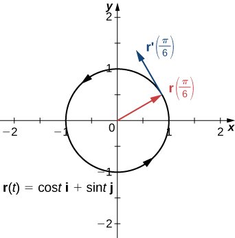
Notice that the vector \vecs{r}′\left(\dfrac{π}{6}\right) is tangent to the circle at the point corresponding to t=\dfrac{π}{6}. This is an example of a tangent vector to the plane curve defined by Equation \ref{eq10}.
Definition: principal unit tangent vector
Let C be a curve defined by a vector-valued function \vecs{r}, and assume that \vecs{r}′(t) exists when t=t_0 A tangent vector \vecs{r} at t=t_0 is any vector such that, when the tail of the vector is placed at point \vecs r(t_0) on the graph, vector \vecs{r} is tangent to curve C. Vector \vecs{r}′(t_0) is an example of a tangent vector at point t=t_0. Furthermore, assume that \vecs{r}′(t)≠0. The principal unit tangent vector at t is defined to be
\vecs{T}(t)=\dfrac{ \vecs{r}′(t)}{‖\vecs{r}′(t)‖},
provided ‖\vecs{r}′(t)‖≠0.
The unit tangent vector is exactly what it sounds like: a unit vector that is tangent to the curve. To calculate a unit tangent vector, first find the derivative \vecs{r}′(t). Second, calculate the magnitude of the derivative. The third step is to divide the derivative by its magnitude.
Example \PageIndex{6}: Finding a Unit Tangent Vector
Find the unit tangent vector for each of the following vector-valued functions:
- \vecs{r}(t)=\cos t \,\hat{\mathbf{i}}+\sin t \,\hat{\mathbf{j}}
- \vecs{u}(t)=(3t^2+2t) \,\hat{\mathbf{i}}+(2−4t^3)\,\hat{\mathbf{j}}+(6t+5)\,\hat{\mathbf{k}}
Solution
-
\begin{array}{lrcl} \text{First step:} & \vecs r′(t) & = & − \sin t \,\hat{\mathbf{i}}+ \cos t \,\hat{\mathbf{j}} \\ \text{Second step:} & ‖\vecs r′(t)‖ & = & \sqrt{(− \sin t)^2+( \cos t)^2} = 1 \\ \text{Third step:} & \vecs T(t) & = & \dfrac{\vecs r′(t)}{‖\vecs r′(t)‖}=\dfrac{− \sin t \,\hat{\mathbf{i}}+ \cos t \,\hat{\mathbf{j}}}{1}=− \sin t \,\hat{\mathbf{i}}+ \cos t \,\hat{\mathbf{j}} \end{array}
\begin{array}{lrcl} \text{First step:} & \vecs r′(t) & = & (6t+2) \,\hat{\mathbf{i}}−12t^2 \,\hat{\mathbf{j}}+6 \,\hat{\mathbf{k}} \\ \text{Second step:} & ‖\vecs r′(t)‖ & = & \sqrt{(6t+2)^2+(−12t^2)^2+6^2} \\ \text{} & \text{} & = & \sqrt{144t^4+36t^2+24t+40} \\ \text{} & \text{} & = & 2 \sqrt{36t^4+9t^2+6t+10} \\ \text{Third step:} & \vecs T(t) & = & \dfrac{\vecs r′(t)}{‖\vecs r′(t)‖}=\dfrac{(6t+2) \,\hat{\mathbf{i}}−12t^2 \,\hat{\mathbf{j}}+6 \,\hat{\mathbf{k}}}{2 \sqrt{36t^4+9t^2+6t+10}} \\ \text{} & \text{} & = & \dfrac{3t+1}{\sqrt{36t^4+9t^2+6t+10}} \,\hat{\mathbf{i}} - \dfrac{6t^2}{\sqrt{36t^4+9t^2+6t+10}} \,\hat{\mathbf{j}} + \dfrac{3}{\sqrt{36t^4+9t^2+6t+10}} \,\hat{\mathbf{k}} \end{array}
Exercise \PageIndex{4}
Find the unit tangent vector for the vector-valued function
\vecs r(t)=(t^2−3)\,\hat{\mathbf{i}}+(2t+1) \,\hat{\mathbf{j}}+(t−2) \,\hat{\mathbf{k}}. \nonumber
- Hint
-
Follow the same steps as in Example \PageIndex{5}.
- Answer
-
\vecs T(t)=\dfrac{2t}{\sqrt{4t^2+5}}\,\hat{\mathbf{i}}+\dfrac{2}{\sqrt{4t^2+5}}\,\hat{\mathbf{j}}+\dfrac{1}{\sqrt{4t^2+5}}\,\hat{\mathbf{k}} \nonumber
Integrals of Vector-Valued Functions
We introduced antiderivatives of real-valued functions in Antiderivatives and definite integrals of real-valued functions in The Definite Integral. Each of these concepts can be extended to vector-valued functions. Also, just as we can calculate the derivative of a vector-valued function by differentiating the component functions separately, we can calculate the antiderivative in the same manner. Furthermore, the Fundamental Theorem of Calculus applies to vector-valued functions as well.
The antiderivative of a vector-valued function appears in applications. For example, if a vector-valued function represents the velocity of an object at time t, then its antiderivative represents position. Or, if the function represents the acceleration of the object at a given time, then the antiderivative represents its velocity.
Definition: Definite and indefinite integrals of vector-valued functions
Let f, g, and h be integrable real-valued functions over the closed interval [a,b].
- The indefinite integral of a vector-valued function \vecs{r}(t)=f(t) \,\hat{\mathbf{i}}+g(t) \,\hat{\mathbf{j}} is
\int [f(t) \,\hat{\mathbf{i}}+g(t) \,\hat{\mathbf{j}}]\,dt= \left[ \int f(t)\,dt \right] \,\hat{\mathbf{i}}+ \left[ \int g(t)\,dt \right] \,\hat{\mathbf{j}}.
The definite integral of a vector-valued function is\int_a^b [f(t) \,\hat{\mathbf{i}}+g(t) \,\hat{\mathbf{j}}]\,dt = \left[ \int_a^b f(t)\,dt \right] \,\hat{\mathbf{i}}+ \left[ \int_a^b g(t)\,dt \right] \,\hat{\mathbf{j}}.
- The indefinite integral of a vector-valued function \vecs r(t)=f(t) \,\hat{\mathbf{i}}+g(t) \,\hat{\mathbf{j}}+h(t) \,\hat{\mathbf{k}} is
\int [f(t) \,\hat{\mathbf{i}}+g(t)\,\hat{\mathbf{j}} + h(t) \,\hat{\mathbf{k}}]\,dt= \left[ \int f(t)\,dt \right] \,\hat{\mathbf{i}}+ \left[ \int g(t)\,dt \right] \,\hat{\mathbf{j}} + \left[ \int h(t)\,dt \right] \,\hat{\mathbf{k}}.
The definite integral of the vector-valued function is\int_a^b [f(t) \,\hat{\mathbf{i}}+g(t) \,\hat{\mathbf{j}} + h(t) \,\hat{\mathbf{k}}]\,dt= \left[ \int_a^b f(t)\,dt \right] \,\hat{\mathbf{i}}+ \left[ \int_a^b g(t)\,dt \right] \,\hat{\mathbf{j}} + \left[ \int_a^b h(t)\,dt \right] \,\hat{\mathbf{k}}.
Since the indefinite integral of a vector-valued function involves indefinite integrals of the component functions, each of these component integrals contains an integration constant. They can all be different. For example, in the two-dimensional case, we can have
\int f(t)\,dt=F(t)+C_1 \; and \; \int g(t)\,dt=G(t)+C_2, \nonumber
where F and G are antiderivatives of f and g, respectively. Then
\begin{align*} \int [f(t) \,\hat{\mathbf{i}}+g(t) \,\hat{\mathbf{j}}]\,dt &= \left[ \int f(t)\,dt \right] \,\hat{\mathbf{i}}+ \left[ \int g(t)\,dt \right] \,\hat{\mathbf{j}} \\[5pt] &= (F(t)+C_1) \,\hat{\mathbf{i}}+(G(t)+C_2) \,\hat{\mathbf{j}} \\[5pt] &=F(t) \,\hat{\mathbf{i}}+G(t) \,\hat{\mathbf{j}}+C_1 \,\hat{\mathbf{i}}+C_2 \,\hat{\mathbf{j}} \\[5pt] &= F(t) \,\hat{\mathbf{i}}+G(t) \,\hat{\mathbf{j}}+\vecs{C} \end{align*}
where \vecs{C}=C_1 \,\hat{\mathbf{i}}+C_2 \,\hat{\mathbf{j}}. Therefore, the integration constants becomes a constant vector.
Example \PageIndex{7}: Integrating Vector-Valued Functions
Calculate each of the following integrals:
- \displaystyle \int [(3t^2+2t) \,\hat{\mathbf{i}}+(3t−6) \,\hat{\mathbf{j}}+(6t^3+5t^2−4) \,\hat{\mathbf{k}}]\,dt
- \displaystyle \int [⟨t,t^2,t^3⟩ \times ⟨t^3,t^2,t⟩] \,dt
- \displaystyle \int_{0}^{\frac{\pi}{3}} [\sin 2t \,\hat{\mathbf{i}}+ \tan t \,\hat{\mathbf{j}}+e^{−2t} \,\hat{\mathbf{k}}]\,dt
Solution
- We use the first part of the definition of the integral of a space curve:
\begin{align*} \int[(3t^2+2t)\,\hat{\mathbf{i}}+(3t−6) \,\hat{\mathbf{j}}+(6t^3+5t^2−4)\,\hat{\mathbf{k}}]\,dt &=\left[\int 3t^2+2t\,dt \right]\,\hat{\mathbf{i}}+ \left[\int 3t−6\,dt \right] \,\hat{\mathbf{j}}+ \left[\int 6t^3+5t^2−4\,dt \right] \,\hat{\mathbf{k}} \\[5pt] &=(t^3+t^2) \,\hat{\mathbf{i}}+\left(\frac{3}{2}t^2−6t\right) \,\hat{\mathbf{j}}+\left(\frac{3}{2}t^4+\frac{5}{3}t^3−4t\right)\,\hat{\mathbf{k}}+\vecs C. \end{align*}
- First calculate ⟨t,t^2,t^3⟩ \times ⟨t^3,t^2,t⟩:
\begin{align*} ⟨t,t^2,t^3⟩ \times ⟨t^3,t^2,t⟩ &= \begin{vmatrix} \hat{\mathbf{i}} & \,\hat{\mathbf{j}} & \,\hat{\mathbf{k}} \\ t & t^2 & t^3 \\ t^3 & t^2 & t \end{vmatrix} \\[5pt] &=(t^2(t)−t^3(t^2)) \,\hat{\mathbf{i}}−(t^2−t^3(t^3))\,\hat{\mathbf{j}}+(t(t^2)−t^2(t^3))\,\hat{\mathbf{k}} \\[5pt] &=(t^3−t^5)\,\hat{\mathbf{i}}+(t^6−t^2)\,\hat{\mathbf{j}}+(t^3−t^5)\,\hat{\mathbf{k}}. \end{align*}
Next, substitute this back into the integral and integrate:\begin{align*} \int [⟨t,t^2,t^3⟩ \times ⟨t^3,t^2,t⟩]\,dt &= \int (t^3−t^5) \,\hat{\mathbf{i}}+(t^6−t^2) \,\hat{\mathbf{j}}+(t^3−t^5)\,\hat{\mathbf{k}}\,dt \\[5pt] &=\left(\frac{t^4}{4}−\frac{t^6}{6}\right)\,\hat{\mathbf{i}}+\left(\frac{t^7}{7}−\frac{t^3}{3}\right)\,\hat{\mathbf{j}}+\left(\frac{t^4}{4}−\frac{t^6}{6}\right)\,\hat{\mathbf{k}}+\vecs C. \end{align*}
- Use the second part of the definition of the integral of a space curve:
\begin{align*} \int_0^{\frac{\pi}{3}} [\sin 2t \,\hat{\mathbf{i}}+ \tan t \,\hat{\mathbf{j}}+e^{−2t} \,\hat{\mathbf{k}}]\,dt &=\left[\int_0^{\frac{π}{3}} \sin 2t \,dt \right] \,\hat{\mathbf{i}}+ \left[ \int_0^{\frac{π}{3}} \tan t \,dt \right] \,\hat{\mathbf{j}}+\left[\int_0^{\frac{π}{3}}e^{−2t}\,dt \right] \,\hat{\mathbf{k}} \\[5pt] &= \left(−\tfrac{1}{2} \cos 2t \right) \Big\vert_{0}^{π/3} \,\hat{\mathbf{i}}−( \ln |\cos t|)\Big\vert_{0}^{π/3} \,\hat{\mathbf{j}}−\left(\tfrac{1}{2}e^{−2t}\right)\Big\vert_{0}^{π/3} \,\hat{\mathbf{k}} \\[5pt] &=\left(−\tfrac{1}{2} \cos \tfrac{2π}{3}+\tfrac{1}{2} \cos 0\right) \,\hat{\mathbf{i}}−\left( \ln \left( \cos \tfrac{π}{3}\right)− \ln( \cos 0)\right) \,\hat{\mathbf{j}}−\left( \tfrac{1}{2}e^{−2π/3}−\tfrac{1}{2}e^{−2(0)}\right) \,\hat{\mathbf{k}} \\[5pt] & =\left(\tfrac{1}{4}+\tfrac{1}{2}\right) \,\hat{\mathbf{i}}−(−\ln 2) \,\hat{\mathbf{j}}−\left(\tfrac{1}{2}e^{−2π/3}−\tfrac{1}{2}\right) \,\hat{\mathbf{k}} \\[5pt] &=\tfrac{3}{4}\,\hat{\mathbf{i}}+(\ln 2) \,\hat{\mathbf{j}}+\left(\tfrac{1}{2}−\tfrac{1}{2}e^{−2π/3}\right)\,\hat{\mathbf{k}}. \end{align*}
Exercise \PageIndex{5}
Calculate the following integral:
\int_1^3 [(2t+4) \,\hat{\mathbf{i}}+(3t^2−4t) \,\hat{\mathbf{j}}]\,dt \nonumber
- Hint
-
Use the definition of the definite integral of a plane curve.
- Answer
-
\int_1^3 [(2t+4) \,\hat{\mathbf{i}}+(3t^2−4t) \,\hat{\mathbf{j}}]\,dt = 16 \,\hat{\mathbf{i}}+10 \,\hat{\mathbf{j}} \nonumber
Integration in the Context of Motion
Above, we defined velocity as the derivative of position and acceleration as the derivative of velocity. Integration allows us to go the other way! As you learned in first semester calculus, integration allows us to generate an object's velocity as a function of time given its acceleration and an initial velocity. We can also find the object's position function by integrating the velocity and using an initial position.
Let's consider an example.
Example \PageIndex{8}: Finding an object's velocity from its acceleration
An object has an acceleration over time given by \vecs a(t) = \sin t \,\hat{\mathbf i} - 2t \,\hat{\mathbf j}, and it's initial velocity was \vecs v(0) = 2 \,\hat{\mathbf i} + \,\hat{\mathbf j}.
a. Find the object's velocity as a function of time.
b. Assuming the object was located at the point (2, 3, -1) when time t = 0, determine the object's position function and find its location at time t = 3 sec.
Solution
a. First, we find the velocity as the antiderivative of the acceleration.
\begin{align*} \vecs v(t) = \int \vecs a(t) \, \,dt &= \int \left( \sin t \,\hat{\mathbf i} - 2t \,\hat{\mathbf j}\right)\,dt \\ &= -\cos t \,\hat{\mathbf i} - t^2\,\hat{\mathbf j} + \vecs C_1 \end{align*}
Now we use the initial velocity to determine \vecs C_1.
\begin{align*} \vecs v(0) = -\cos 0 \,\hat{\mathbf i} - (0)^2\,\hat{\mathbf j} + \vecs C_1 &= 2 \,\hat{\mathbf i} + \,\hat{\mathbf j} \\ -\hat{\mathbf i} + \vecs C_1 &= 2 \,\hat{\mathbf i} + \,\hat{\mathbf j} \\ \\ \text{And so} \quad \vecs C_1 &= 3 \,\hat{\mathbf i} + \,\hat{\mathbf j} \end{align*}
Incorporating this constant vector into our velocity function from above, we obtain the velocity describing this object's motion over time:
\vecs v(t) = \left( 3 -\cos t \right) \,\hat{\mathbf i} + \left(1 - t^2\right) \,\hat{\mathbf j}
b. Since the object's position is at the point (2, 3, -1) when time t = 0, we know \vecs r(0) = 2 \,\hat{\mathbf i} + 3 \,\hat{\mathbf j} - \,\hat{\mathbf k}.
Now, to determine the object's position function, we integrate it's velocity.
\begin{align*} \vecs r(t) = \int \vecs v(t) \, \,dt &= \int \bigg[\left( 3 -\cos t \right) \,\hat{\mathbf i} + \left(1 - t^2\right) \,\hat{\mathbf j}\bigg]\,dt \\ &= \left( 3t -\sin t \right) \,\hat{\mathbf i} + \left(t - \frac{t^3}{3}\right) \,\hat{\mathbf j} + \vecs C_2 \end{align*}
Now we use the initial position to determine \vecs C_2.
\begin{align*} \vecs r(0) = \left( 3(0) -\sin 0 \right) \,\hat{\mathbf i} + \left( 0 - \frac{(0)^3}{3}\right) \,\hat{\mathbf j} + \vecs C_2 &= 2 \,\hat{\mathbf i} + 3 \,\hat{\mathbf j} - \,\hat{\mathbf k}\\ \\ \text{And so} \quad \vecs C_2 &= 2 \,\hat{\mathbf i} + 3 \,\hat{\mathbf j} - \,\hat{\mathbf k} \end{align*}
Incorporating this constant vector into our position function from above, we obtain:
\vecs r(t) = \left( 2 + 3t -\sin t \right) \,\hat{\mathbf i} + \left(3 + t - \frac{t^3}{3}\right) \,\hat{\mathbf j} - \,\hat{\mathbf k}
To find the object's position at time t = 3 seconds, we just evaluate this position function at t = 3.
\begin{align*} \vecs r(3) &= \left( 2 + 3(3) -\sin 3 \right) \,\hat{\mathbf i} + \left(3 + 3 - \frac{(3)^3}{3}\right) \,\hat{\mathbf j} - \,\hat{\mathbf k} \\ &= \left( 11 -\sin 3 \right) \,\hat{\mathbf i} - 3 \,\hat{\mathbf j} - \,\hat{\mathbf k} \end{align*}
This position vector indicates that the object will be located at the point (11 -\sin 3, -3, -1) at time t = 3 seconds.
The Meaning of Definite Integrals of Vector-Valued Functions
Now let's turn our attention to the meaning of a definite integral of a vector-valued function. The context in which this will make the most sense is where the function we integrate is a velocity function. That is,
\int_a^b \vecs v(t) \, \,dt
We know that the antiderivative of velocity is position and that this definite integral gives us the change in position over the time interval, a \le t\le b. In other words,
\int_a^b \vecs v(t) \, \,dt = \vecs r(b) - \vecs r(a)
Thus, the definite integral of velocity over a time interval a \le t\le b gives us the displacement vector that indicates the change in position over this time interval.
In general, the definite integral
\displaystyle \int_a^b \vecs r(t) \, \,dt = \vecs q(b) - \vecs q(a), where \vecs q(t) is the antiderivative of \vecs r(t),
gives us a change in the antiderivative of our vector-valued function over the given inteval [a,b]. This will always be a constant vector that would fit from tip to tip of the vectors given by the antiderivative function at t = a and t = b, respectively (assuming the vectors were placed in standard position).
Summary
- To calculate the derivative of a vector-valued function, calculate the derivatives of the component functions, then put them back into a new vector-valued function.
- Many of the properties of differentiation of scalar functions also apply to vector-valued functions.
- The derivative of a vector-valued function \vecs r(t) is also a tangent vector to the curve. The unit tangent vector \vecs T(t) is calculated by dividing the derivative of a vector-valued function by its magnitude.
- The antiderivative of a vector-valued function is found by finding the antiderivatives of the component functions, then putting them back together in a vector-valued function.
- The definite integral of a vector-valued function is found by finding the definite integrals of the component functions, then putting them back together in a vector-valued function.
Key Equations
- Derivative of a vector-valued function\vecs r′(t) = \lim \limits_{\Delta t \to 0} \dfrac{\vecs r(t+\Delta t)−\vecs r(t)}{ \Delta t} \nonumber
- Principal unit tangent vector \vecs T(t)=\frac{\vecs r′(t)}{‖\vecs r′(t)‖}
- Indefinite integral of a vector-valued function \int [f(t) \,\hat{\mathbf{i}}+g(t)\,\hat{\mathbf{j}} + h(t) \,\hat{\mathbf{k}}]\,dt= \left[ \int f(t)\,dt \right] \,\hat{\mathbf{i}}+ \left[ \int g(t)\,dt \right] \,\hat{\mathbf{j}} + \left[ \int h(t)\,dt \right] \,\hat{\mathbf{k}}\nonumber
- Definite integral of a vector-valued function \int_a^b [f(t) \,\hat{\mathbf{i}}+g(t) \,\hat{\mathbf{j}} + h(t) \,\hat{\mathbf{k}}]\,dt= \left[\int_a^b f(t)\,dt \right] \,\hat{\mathbf{i}}+ \left[ \int _a^b g(t)\,dt \right] \,\hat{\mathbf{j}} + \left[ \int _a^b h(t)\,dt \right] \,\hat{\mathbf{k}}\nonumber
Glossary
- definite integral of a vector-valued function
- the vector obtained by calculating the definite integral of each of the component functions of a given vector-valued function, then using the results as the components of the resulting function
- derivative of a vector-valued function
- the derivative of a vector-valued function \vecs{r}(t) is \vecs{r}′(t) = \lim \limits_{\Delta t \to 0} \frac{\vecs r(t+\Delta t)−\vecs r(t)}{ \Delta t}, provided the limit exists
- indefinite integral of a vector-valued function
- a vector-valued function with a derivative that is equal to a given vector-valued function
- principal unit tangent vector
- a unit vector tangent to a curve C
- tangent vector
- to \vecs{r}(t) at t=t_0 any vector \vecs v such that, when the tail of the vector is placed at point \vecs r(t_0) on the graph, vector \vecs{v} is tangent to curve C
Contributors
Gilbert Strang (MIT) and Edwin “Jed” Herman (Harvey Mudd) with many contributing authors. This content by OpenStax is licensed with a CC-BY-SA-NC 4.0 license. Download for free at http://cnx.org.
- Paul Seeburger (Monroe Community College) edited this section and added content on visualizing the derivative of a vector-valued function and content on smooth vector-valued functions.