2.5: Transcendental Functions

The transcendental functions include the trigonometric functions $\sin x$, $\cos x$, $\tan x$, the exponential function $e^{x}$, and the natural logarithm function $\ln x$. These functions are developed in detail in Chapters 7 and 8. This section contains a brief discussion.

1. Trignometric Functions

The Greek letters $\theta$ (theta) and $\phi$ (phi) are often used for angles. In the calculus it is convenient to measure angles in radians instead of degrees. An angle $\theta$ in radians is defined as the length of the arc of the angle on a circle of radius one (Figure $\PageIndex{1}$). Since a circle of radius one has circumference $2 \pi$, $$360 \ \text{degrees} = 2\pi \ \text{radians} \nonumber$$

Figure $\PageIndex{1}$. Angle in radians defined as length of arc on a unit circle.

Thus a right angle is $$90 \ \text{degrees} = \pi/2 \ \text{radians}. \nonumber$$

To define the sine and cosine functions, we consider a point $P(x, y)$ on the unit circle $x^{2} + y^{2} = 1$. Let $\theta$ be the angle measured counterclockwise in radians from the point $(1, 0)$ to the point $P(x, y)$ as shown in Figure $\PageIndex{2}$. Both coordinates $x$ and $y$ depend on $\theta$. The value of $x$ is called the cosine of $\theta$, and the value of $y$ is the sine of $\theta$. In symbols, $$x = \cos \theta, \quad y = \sin \theta. \nonumber$$ The tangent of $\theta$ is defined by $$\tan \theta = \sin \theta / \cos \theta. \nonumber$$

Figure $\PageIndex{2}$: Sine and cosine functions defined using the unit circle.

Negative angles and angles greater than $2 \pi$ radians are also allowed. The trigonometric functions can also be defined using the sides of a right triangle, but this method only works for $\theta$ between $0$ and $\pi/2$. Let $\theta$ be one of the acute angles of a right triangle as shown in Figure $\PageIndex{3}$.

Figure $\PageIndex{3}$: Right triangle for use in defining trigonometric functions.

Then $$\begin{align*} \sin \theta &= \frac{\text{opposite side}}{\text{hypotenuse}} = \frac{a}{c}, \\[4pt] \cos \theta &= \frac{\text{adjacent side}}{\text{hypotenuse}} = \frac{b}{c}, \\[4pt] \tan \theta &= \frac{\text{opposite side}}{\text{adjacent side}} = \frac{a}{b}. \end{align*}$$

The two definitions, with circles and right triangles, can be seen to be equivalent using similar triangles.

Table $\PageIndex{1}$ gives the values of $\sin \theta$ and $\cos \theta$ for some important values of $\theta$.

Table $\PageIndex{1}$. $\sin \theta$ and $\cos \theta$ at important values of $\theta$.

$\theta$ in degrees	$0^{\circ}$	$30^{\circ}$	$45^{\circ}$	$60^{\circ}$	$90^{\circ}$	$180^{\circ}$	$270^{\circ}$	$360^{\circ}$
$\theta$ in radians	$0$	$\pi/6$	$\pi/4$	$\pi/3$	$\pi/2$	$\pi$	$3 \pi/2$	$2 \pi$
$\sin \theta$	$0$	$1/2$	$\sqrt{2}/2$	$\sqrt{3}/2$	$1$	$0$	$-1$	$0$
$\cos \theta$	$1$	$\sqrt{3}/2$	$\sqrt{2}/2$	$1/2$	$0$	$1$	$0$	$1$

A useful identity which follows from the unit circle equation $x^{2} + y^{2} = 1$ is $$\sin^{2} \theta + \cos^{2} \theta = 1. \nonumber$$

Here $\sin^{2} \theta$ means $(\sin \theta)^{2}$.

Figure $\PageIndex{4}$ shows the graphs of $\sin \theta$ and $\cos \theta$, which look like waves that oscillate between $1$ and $-1$ and repeat every $2 \pi$ radians.

The derivatives of the sine and cosine functions are: $$\begin{align*} \frac{d (\sin \theta)}{d \theta} &= \cos \theta. \\[4pt] \frac{d (\cos \theta)}{d \theta} &= - \sin \theta. \end{align*}$$

Figure $\PageIndex{4}$: Graphs of $\sin \theta$ and $\cos \theta$.

In both formulas $\theta$ is measured in radians. We can see intuitively why these are the derivatives in Figure $\PageIndex{5}$.

In the triangle under the infinitesimal microscope, $$\begin{align*} \frac{\Delta (\sin \theta)}{\Delta \theta} &\approx \frac{\text{adjacent side}}{\text{hypotenuse}} = \cos \theta; \\[4pt] \frac{\Delta (\cos \theta)}{\Delta \theta} &\approx \frac{- \text{opposite side}}{\text{hypotenuse}} = - \sin \theta \end{align*}$$

Figure $\PageIndex{5}$.

Notice that $\cos \theta$ decreases, and $\Delta (cos \theta)$ is negative in the figure, so the derivative of $\cos \theta$ is $- \sin \theta$ instead of just $\sin \theta$.

Using the rules of differentiation we can find other derivatives.

Example $\PageIndex{1}$

Differentiate $y = \sin^{2} \theta$.

Solution

Let $u = \sin \theta$, $y = u^{2}$. Then $$\frac{dy}{d \theta} = 2u \frac{du}{d \theta} = 2 \sin \theta \cos \theta. \nonumber$$

Example $\PageIndex{2}$

Differentiate $y = \sin \theta (1 - \cos \theta)$.

Solution

Let $u = \sin \theta$, $v = 1 - \cos \theta$. Then $y = u \cdot v$, and $$\begin{align*} \frac{dy}{d \theta} = u \frac{dv}{d \theta} + v \frac{du}{d \theta} &= \sin \theta (-(- \sin \theta)) + (1 - \cos \theta) \cos \theta \\ &= \sin^{2} \theta + \cos \theta - \cos^{2} \theta. \end{align*}$$

The other trigonometric functions (the secant, cosecant, and cotangent functions) and the inverse trigonometric functions are discussed in Chapter 7.

2. Exponential Functions

Given a positive real number $b$ and a rational number $m/n$, the rational power $b^{m/n}$ is defined as $$b^{m/n} = \sqrt[n]{b^{m}}, \nonumber$$ the positive $n$th root of $b^{m}$. The negative power $b^{-m/n}$ is $$b^{-m/n} = \frac{1}{b^{m/n}}. \nonumber$$

As an example consider $b = 10$. Several values of $10^{m/n}$ are shown in Table $\PageIndex{2}$.

Table $\PageIndex{2}$.

$10^{-3}$	$10^{-3/2}$	$10^{-1}$	$10^{-2/3}$	$10^{-1/3}$	$10^{0}$	$10^{1/3}$	$10^{2/3}$	$10^{1}$	$10^{3/2}$	$10^{3}$
$\dfrac{1}{1000}$	$\dfrac{1}{10 \sqrt{10}}$	$\dfrac{1}{10}$	$\dfrac{1}{\sqrt[3]{100}}$	$\dfrac{1}{\sqrt[3]{10}}$	$1$	$\sqrt[3]{10}$	$\sqrt[3]{100}$	$10$	$10 \sqrt{10}$	$1000$

If we plot all the rational powers $10^{m/n}$, we get a dotted line, with one value for each rational number $m/n$, as in Figure $\PageIndex{6}$.

Figure $\PageIndex{6}$: Plotted values of several rational $x$ values of $10^{x}$.

By connecting the dots with a smooth curve, we obtain a function $y = 10^{x}$, where $x$ varies over all real numbers instead of just the rationals. $10^{x}$ is called the
exponential function with base 10. It is positive for all $x$ and follows the rules $$10^{a + b} = 10^{a} \cdot 10^{b}, \quad 10^{a \cdot b} = \left(10^{a}\right)^{b}. \nonumber$$

The derivative of $10^{x}$ is a constant times $10^{x}$, approximately $$\frac{d \left(10^{x}\right)}{dx} \sim (2.303) 10^{x}. \nonumber$$

To see this let $\Delta x$ be a nonzero infinitesimal. Then $$\frac{d \left(10^{x}\right)}{dx} = st \left[\frac{10^{x + \Delta x} - 10^{x}}{\Delta x}\right] = st \left[\frac{\left(10^{x} - 1\right) 10^{x}}{\Delta x}\right] = st \left[\frac{10^{\Delta x} - 1}{\Delta x}\right] 10^{x}. \nonumber$$

The number $st \left[ \left(10^{\Delta x} - 1\right)/\Delta x\right]$ is a constant which does not depend on $x$ and can be shown to be approximately $2.303$.

If we start with a given positive real number $b$ instead of $10$, we obtain the exponential function with base $b$, $y = b^{x}$. The derivative of $b^{x}$ is equal to the constant $st \left[ \left(b^{\Delta x} - 1\right)/\Delta x\right]$ times $b^{x}$. This constant depends on $b$. The derivative is computed as follows: $$\frac{d \left(b^{x}\right)}{dx} = st \left[\frac{b^{x + \Delta x} - b^{x}}{\Delta x}\right] = st \left[\frac{\left(b^{\Delta x} - 1\right) b^{x}}{\Delta x}\right] = st \left[\frac{b^{\Delta x} - 1}{\Delta x}\right] b^{x}. \nonumber$$

The most useful base for the calculus is the number $e$. $e$ is defined as the real number such that the derivative of $e^{x}$ is $e^{x}$ itself, $$\frac{d \left(e^{x}\right)}{dx} = e^{x}. \nonumber$$

In other words, $e$ is the real number such that the constant $$st \left[\frac{e^{\Delta x} - 1}{\Delta x}\right] = 1. \nonumber$$ (where $\Delta x$ is a nonzero infinitesimal). It will be shown in Section 8.3 that there is such a number $e$ and that $e$ has the approximate value $$e \sim 2.71828. \nonumber$$

The function $y = e^{x}$ is called the exponential function. $e^{x}$ is always positive and follows the rules $$e^{a + b} = e^{a} \cdot e^{b}, \quad e^{a \cdot b} = \left(e^{a}\right)^{b}, \quad e^{0} = 1. \nonumber$$

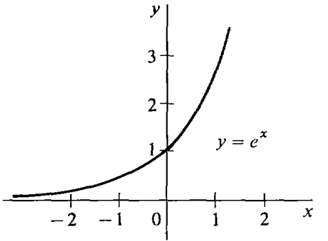
Figure $\PageIndex{7}$ shows the graph of $y = e^{x}$.

Figure $\PageIndex{7}$: Graph of $y = e^{x}$.

Example $\PageIndex{3}$

Find the derivative of $y = x^{2} e^{x}$.

Solution

By the Product Rule, $$\frac{dy}{dx} = x^{2} \frac{d \left(e^{x}\right)}{dx} + e^{x} \frac{d \left(x^{2}\right)}{dx} = x^{2} e^{x} + 2x e^{x}. \nonumber$$

3. The Natural Logarithm

The inverse of the exponential function $x = e^{y}$ is the natural logarithm function, written $$y = \ln x. \nonumber$$

Verbally, $\ln x$ is the number y such that $e^{y} = x$. Since $y = \ln x$ is the inverse function of $x = e^{y}$, we have $$e^{\ln a} = a, \quad \ln \left(e^{a}\right) = a. \nonumber$$

The simplest values of $y = \ln x$ are $$\ln (1/e) = -1, \quad \ln (1) = 0, \quad \ln e = 1. \nonumber$$

Figure $\PageIndex{8}$ shows the graph of $y = \ln x$. It is defined only for $x > 0$.

Figure $\PageIndex{8}$: Graph of $y = \ln x$.

The most important rules for logarithms are $$\begin{align*} \ln(ab) &= \ln a + \ln b, \\ \ln (ab) &= b \cdot \ln a. \end{align*}$$

The natural logarithm function is important in calculus because its derivative is simply $1/x$, $$\frac{d (\ln x)}{dx} = \frac{1}{x}, \quad (x > 0). \nonumber$$

This can be derived from the Inverse Function Rule.

If $y = \ln x$, then $$\begin{align*} x &= e^{y}, \\ \frac{dx}{dy} &= e^{y}, \\ \frac{dy}{dx} &= \frac{1}{dx/dy} = \frac{1}{e^{y}} = \frac{1}{x}. \end{align*}$$

The natural logarithm is also called the logarithm to the base $e$ and is sometimes written $\log_{e} x$. Logarithms to other bases are discussed in Chapter 8.

Example $\PageIndex{4}$

Differentiate $y = \dfrac{1}{\ln x}$.

Solution

$$\frac{dy}{dx} = \frac{-1}{(\ln x)^{2}} \frac{d (\ln x)}{dx} = \frac{-1}{x (\ln x)^{2}}. \nonumber$$

4. Summary

Here is a list of the new derivatives given in this section. $$\begin{align*} \frac{d (\sin x)}{dx} &= \cos x, \\[4pt] \frac{d (\cos x)}{dx} &= - \sin x, \\[4pt] \frac{d e^{x}}{dx} &= e^{x}, \\[4pt] \frac{d (\ln x)}{dx} &= \frac{1}{x} \quad (x > 0). \end{align*}$$

Tables of values for $\sin x$, $\cos x$, $e^{x}$, and $\ln x$ can be found at the end of the book.

Problems for Section 2.5

In Problems 1-20, find the derivative.

1.	$y = \cos^{2} \theta$	2.	$s = \tan^{2} t$
3.	$y = 2 \sin x + 3 \cos x$	4.	$y = \sin x \cdot \cos x$
5.	$w = \frac{1}{\cos z}$	6.	\(w = \dfrac{1}{\sin z\)
7.	$y = \sin^{n} \theta$	8.	$y = \tan^{n} \theta$
9.	$s = t \sin t$	10.	$s = \dfrac{\cos t}{t - 1}$
11.	$y = xe^{x}$	12.	$y = 1/\left(1 + e^{x}\right)$
13.	$y = (\ln x)^{2}$	14.	$y = x \ln x$
15.	$y = e^{x} \cdot \ln x$	16.	$y = e^{x} \cdot \sin x$
17.	$u = \sqrt{v} \left(1 - e^{n}\right)$	18.	$u = \left(1 + e^{v}\right) \left(1 - e^{v}\right)$
19.	$y = x^{n} \ln x$	20.	$y = (\ln x)^{n}$

In Problems 21-24, find the equation of the tangent line at the given point.

21.	$y = \sin x \text{ at } (\pi/6, 1/2)$	22.	$s = \cos x \text{ at } (\pi/4, \sqrt{2}/2)$
23.	$y = x - \ln x \text{ at } (e, e-1)$	24.	$y = e^{-x} \text{ at } (0, 1)$