5.3: Applications of Polynomials

Last updated
Save as PDF

Page ID: 19879

$ \newcommand{\vecs}[1]{\overset { \scriptstyle \rightharpoonup} {\mathbf{#1}} } $

$ \newcommand{\vecd}[1]{\overset{-\!-\!\rightharpoonup}{\vphantom{a}\smash {#1}}} $

$ \newcommand{\id}{\mathrm{id}}$ $ \newcommand{\Span}{\mathrm{span}}$

( \newcommand{\kernel}{\mathrm{null}\,}\) $ \newcommand{\range}{\mathrm{range}\,}$

$ \newcommand{\RealPart}{\mathrm{Re}}$ $ \newcommand{\ImaginaryPart}{\mathrm{Im}}$

$ \newcommand{\Argument}{\mathrm{Arg}}$ $ \newcommand{\norm}[1]{\| #1 \|}$

$ \newcommand{\inner}[2]{\langle #1, #2 \rangle}$

$ \newcommand{\Span}{\mathrm{span}}$

$ \newcommand{\id}{\mathrm{id}}$

$ \newcommand{\Span}{\mathrm{span}}$

$ \newcommand{\kernel}{\mathrm{null}\,}$

$ \newcommand{\range}{\mathrm{range}\,}$

$ \newcommand{\RealPart}{\mathrm{Re}}$

$ \newcommand{\ImaginaryPart}{\mathrm{Im}}$

$ \newcommand{\Argument}{\mathrm{Arg}}$

$ \newcommand{\norm}[1]{\| #1 \|}$

$ \newcommand{\inner}[2]{\langle #1, #2 \rangle}$

$ \newcommand{\Span}{\mathrm{span}}$ $ \newcommand{\AA}{\unicode[.8,0]{x212B}}$

$ \newcommand{\vectorA}[1]{\vec{#1}} % arrow$

$ \newcommand{\vectorAt}[1]{\vec{\text{#1}}} % arrow$

$ \newcommand{\vectorB}[1]{\overset { \scriptstyle \rightharpoonup} {\mathbf{#1}} } $

$ \newcommand{\vectorC}[1]{\textbf{#1}} $

$ \newcommand{\vectorD}[1]{\overrightarrow{#1}} $

$ \newcommand{\vectorDt}[1]{\overrightarrow{\text{#1}}} $

$ \newcommand{\vectE}[1]{\overset{-\!-\!\rightharpoonup}{\vphantom{a}\smash{\mathbf {#1}}}} $

$ \newcommand{\vecs}[1]{\overset { \scriptstyle \rightharpoonup} {\mathbf{#1}} } $

$ \newcommand{\vecd}[1]{\overset{-\!-\!\rightharpoonup}{\vphantom{a}\smash {#1}}} $

$\newcommand{\avec}{\mathbf a}$ $\newcommand{\bvec}{\mathbf b}$ $\newcommand{\cvec}{\mathbf c}$ $\newcommand{\dvec}{\mathbf d}$ $\newcommand{\dtil}{\widetilde{\mathbf d}}$ $\newcommand{\evec}{\mathbf e}$ $\newcommand{\fvec}{\mathbf f}$ $\newcommand{\nvec}{\mathbf n}$ $\newcommand{\pvec}{\mathbf p}$ $\newcommand{\qvec}{\mathbf q}$ $\newcommand{\svec}{\mathbf s}$ $\newcommand{\tvec}{\mathbf t}$ $\newcommand{\uvec}{\mathbf u}$ $\newcommand{\vvec}{\mathbf v}$ $\newcommand{\wvec}{\mathbf w}$ $\newcommand{\xvec}{\mathbf x}$ $\newcommand{\yvec}{\mathbf y}$ $\newcommand{\zvec}{\mathbf z}$ $\newcommand{\rvec}{\mathbf r}$ $\newcommand{\mvec}{\mathbf m}$ $\newcommand{\zerovec}{\mathbf 0}$ $\newcommand{\onevec}{\mathbf 1}$ $\newcommand{\real}{\mathbb R}$ $\newcommand{\twovec}[2]{\left[\begin{array}{r}#1 \\ #2 \end{array}\right]}$ $\newcommand{\ctwovec}[2]{\left[\begin{array}{c}#1 \\ #2 \end{array}\right]}$ $\newcommand{\threevec}[3]{\left[\begin{array}{r}#1 \\ #2 \\ #3 \end{array}\right]}$ $\newcommand{\cthreevec}[3]{\left[\begin{array}{c}#1 \\ #2 \\ #3 \end{array}\right]}$ $\newcommand{\fourvec}[4]{\left[\begin{array}{r}#1 \\ #2 \\ #3 \\ #4 \end{array}\right]}$ $\newcommand{\cfourvec}[4]{\left[\begin{array}{c}#1 \\ #2 \\ #3 \\ #4 \end{array}\right]}$ $\newcommand{\fivevec}[5]{\left[\begin{array}{r}#1 \\ #2 \\ #3 \\ #4 \\ #5 \\ \end{array}\right]}$ $\newcommand{\cfivevec}[5]{\left[\begin{array}{c}#1 \\ #2 \\ #3 \\ #4 \\ #5 \\ \end{array}\right]}$ $\newcommand{\mattwo}[4]{\left[\begin{array}{rr}#1 \amp #2 \\ #3 \amp #4 \\ \end{array}\right]}$ $\newcommand{\laspan}[1]{\text{Span}\{#1\}}$ $\newcommand{\bcal}{\cal B}$ $\newcommand{\ccal}{\cal C}$ $\newcommand{\scal}{\cal S}$ $\newcommand{\wcal}{\cal W}$ $\newcommand{\ecal}{\cal E}$ $\newcommand{\coords}[2]{\left\{#1\right\}_{#2}}$ $\newcommand{\gray}[1]{\color{gray}{#1}}$ $\newcommand{\lgray}[1]{\color{lightgray}{#1}}$ $\newcommand{\rank}{\operatorname{rank}}$ $\newcommand{\row}{\text{Row}}$ $\newcommand{\col}{\text{Col}}$ $\renewcommand{\row}{\text{Row}}$ $\newcommand{\nul}{\text{Nul}}$ $\newcommand{\var}{\text{Var}}$ $\newcommand{\corr}{\text{corr}}$ $\newcommand{\len}[1]{\left|#1\right|}$ $\newcommand{\bbar}{\overline{\bvec}}$ $\newcommand{\bhat}{\widehat{\bvec}}$ $\newcommand{\bperp}{\bvec^\perp}$ $\newcommand{\xhat}{\widehat{\xvec}}$ $\newcommand{\vhat}{\widehat{\vvec}}$ $\newcommand{\uhat}{\widehat{\uvec}}$ $\newcommand{\what}{\widehat{\wvec}}$ $\newcommand{\Sighat}{\widehat{\Sigma}}$ $\newcommand{\lt}{<}$ $\newcommand{\gt}{>}$ $\newcommand{\amp}{&}$ $\definecolor{fillinmathshade}{gray}{0.9}$

In this section we investigate real-world applications of polynomial functions.

Example $\PageIndex{1}$

The average price of a gallon of gas at the beginning of each month for the period starting in November 2010 and ending in May 2011 are given in the margin. The data is plotted in Figure $\PageIndex{1}$ and ﬁtted with the following third degree polynomial, where t is the number of months that have passed since October of 2010.

\[p(t)=-0.0080556 t^{3}+0.11881 t^{2}-0.30671 t+3.36 \label{Eq5.3.1} \]

Use the graph and then the polynomial to estimate the price of a gallon of gas in California in February 2011.

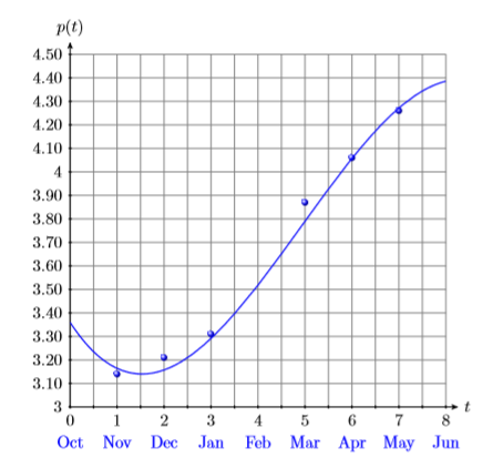
fig 5.3.1.png — Figure $\PageIndex{1}$: Fitting gas price versus month with a cubic polynomial.

\[\begin{array}{c|c}\hline \text { Month } & {\text { Price }} \\ \hline \text { Nov. } & {3.14} \\ {\text { Dec. }} & {3.21} \\ {\text { Jan }} & {3.31} \\ {\text { Mar. }} & {3.87} \\ {\text { Apr. }} & {4.06} \\ {\text { May }} & {4.26} \\ \hline\end{array} \nonumber \]

Solution

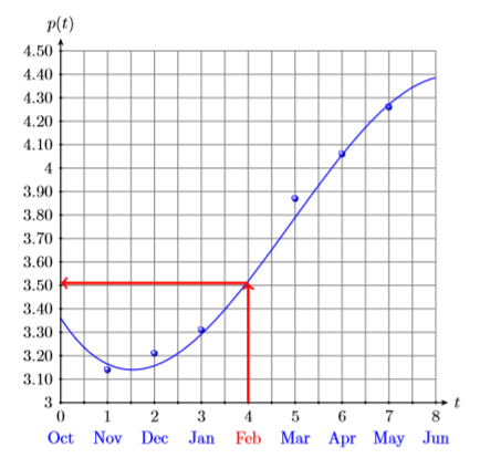
Locate February ($t = 4$) on the horizontal axis. From there, draw a vertical arrow up to the graph, and from that point of intersection, a second horizontal arrow over to the vertical axis (see Figure $\PageIndex{2}$). It would appear that the price per gallon in February was approximately $\$3.51$.

fig 5.3.2.png — Figure $\PageIndex{2}$: Approximating price of gas during February.

Next, we’ll use the ﬁtted third degree polynomial to approximate the price per gallon for the month of February, 2011. Start with the function deﬁned by Equation \ref{Eq5.3.1} and substitute $4$ for $t$.

\[\begin{aligned} p(t) &=-0.0080556 t^{3}+0.11881 t^{2}-0.30671 t+3.36 \\ p(4) &=-0.0080556(4)^{3}+0.11881(4)^{2}-0.30671(4)+3.36 \end{aligned} \nonumber \]

Use the calculator to evaluate $p(4)$ (see Figure $\PageIndex{3}$). Rounding to the nearest

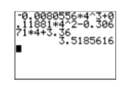
fig 5.3.3.png — Figure $\PageIndex{3}$: Evaluating $p(4)$.

penny, the price in February was $\$3.52$ per gallon.

Example $\PageIndex{2}$

If a projectile is ﬁred into the air, its height above ground at any time is given by the formula

\[y=y_{0}+v_{0} t-\dfrac{1}{2} g t^{2} \label{Eq5.3.2} \]

where

$y$ = height above ground at time $t$

$y_0$ = initial height above ground at time $t = 0$

$v_0$ = initial velocity at time $t = 0$

$g$ = acceleration due to gravity

$t$ = time passed since projectile’s ﬁring

If a projectile is launched with an initial velocity of $100$ meters per second ($100$m/s) from a rooftop $8$ meters ($8$m) above ground level, at what time will the projectile ﬁrst reach a height of $400$ meters ($400$m)? Note: Near the earth’s surface, the acceleration due to gravity is approximately $9.8$ meters per second per second ($9.8$(m/s)/s or $9.8$m/s²).

Solution

We’re given the initial height is $y_0 = 8$m, the initial velocity is $v_0 = 100$m/s, and the acceleration due to gravity is $g =9.8$m/s². Substitute these values in Equation \ref{Eq5.3.2}, then simplify to produce the following result:

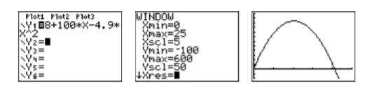
\[\begin{array}{l}{y=y_{0}+v_{0} t-\dfrac{1}{2} g t^{2}} \\ {y=8+100 t-\dfrac{1}{2}(9.8) t^{2}} \\ {y=8+100 t-4.9 t^{2}}\end{array} \nonumber \]

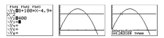
Enter $y=8+100 t-4.9 t^{2}$ as $\mathbf{Y} \mathbf{1}=\mathbf{8}+100^{*} \mathbf{X}-4.9^{*} \mathbf{X} \wedge \mathbf{2}$ in the Y= menu (see the ﬁrst image in Figure $\PageIndex{4}$). After some experimentation, we settled on the WINDOW parameters shown in the second image in Figure $\PageIndex{4}$. Push the GRAPH button to produce the graph of $y=8+100 t-4.9 t^{2}$ shown in the third image Figure $\PageIndex{4}$.

In this example, the horizontal axis is actually the $t$-axis. So when we set $\mathrm{Xmin}$ and $\mathrm{Xmax}$, we’re actually setting bounds on the $t$-axis.

fig 5.3.4.png — Figure $\PageIndex{4}$: Sketching the graph of $y = 8 + 100t−4.9t^2$.

To ﬁnd when the projectile reaches a height of $400$ meters ($400$m), substitute $400$ for $y$ to obtain:

\[400=8+100 t-4.9 t^{2} \label{Eq5.3.3} \]

Enter the left-hand side of Equation \ref{Eq5.3.3} into $\mathbf{Y} \boldsymbol{2}$ in the Y= menu, as shown in the ﬁrst image in Figure $\PageIndex{5}$. Push the GRAPH button to produce the result shown in the second image in Figure $\PageIndex{5}$. Note that there are two points of intersection, which makes sense as the projectile hits $400$ meters on the way up and $400$ meters on the way down.

fig 5.3.5.png — Figure $\PageIndex{5}$: Determining when the object ﬁrst reaches $400$ meters.

To ﬁnd the ﬁrst point of intersection, select 5:intersect from the CALC menu. Press ENTER in response to “First curve,” then press ENTER again in response to “Second curve.” For your guess, use the arrow keys to move the cursor closer to the ﬁrst point of intersection than the second. At this point, press ENTER in response to “Guess.” The result is shown in the third image in Figure $\PageIndex{5}$. The projectile ﬁrst reaches a height of $400$ meters at approximately $5.2925359$ seconds after launch.

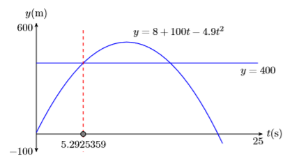
fig 5.3.6.png — Figure $\PageIndex{6}$: Reporting your graphical solution on your homework.

The parabola shown in Figure $\PageIndex{6}$ is not the actual ﬂight path of the projectile. The graph only predicts the height of the projectile as a function of time.

Reporting the solution on your homework: Duplicate the image in your calculator’s viewing window on your homework page. Use a ruler to draw all lines, but freehand any curves.

Label the horizontal and vertical axes with $t$ and $y$, respectively (see Figure $\PageIndex{6}$). Include the units (seconds (s) and meters (m)).
Place your WINDOW parameters at the end of each axis (see Figure $\PageIndex{6}$). Include the units (seconds (s) and meters (m)).
Label each graph with its equation (see Figure $\PageIndex{6}$).
Draw a dashed vertical line through the ﬁrst point of intersection. Shade and label the point (with its $t$-value) where the dashed vertical line crosses the $t$-axis. This is the ﬁrst solution of the equation $400 = 8+100t−4.9t^2$ (see Figure $\PageIndex{6}$).

Rounding to the nearest tenth of a second, it takes the projectile approximately $t ≈ 5.3$ seconds to ﬁrst reach a height of $400$ meters.

The phrase “shade and label the point” means ﬁll in the point on the $t$-axis, then write the $t$-value of the point just below the shaded point.

Exercise $\PageIndex{2}$

If a projectile is launched with an initial velocity of $60$ meters per second from a rooftop $12$ meters above ground level, at what time will the projectile ﬁrst reach a height of $150$ meters?

Answer: $\approx 3.0693987$ seconds

Zeros and $x$-intercepts of a Function

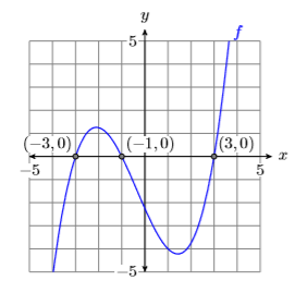
Recall that $f(x)$ and $y$ are interchangeable. Therefore, if we are asked to ﬁnd where a function is equal to zero, then we need to ﬁnd the points on the graph of the function that have a $y$-value equal to zero (see Figure $\PageIndex{7}$).

fig 5.3.7.png — Figure $\PageIndex{7}$: Locating the zeros of a function.

Zeros and $x$-intercepts

The points where the graph off crosses the $x$-axis are called the $x$-intercepts of the graph of $f$. The $x$-value of each $x$-intercept is called a zero of the function $f$.

The graph of $f$ crosses the $x$-axis in Figure $\PageIndex{7}$ at $(−3,0)$, $(−1,0)$, and $(3 ,0)$. Therefore:

The $x$-intercepts of f are: $(−3,0)$, $(−1,0)$, and $(3,0)$
The zeros of $f$ are: $−3$, $−1$, and $3$

Key idea

A function is zero where its graph crosses the $x$-axis.

Example $\PageIndex{3}$

Find the zero(s) of the function $f(x)=1 .5x +5 .25$.

Solution

Remember, $f(x)=1 .5x +5 .25$ and $y =1 .5x +5 .25$ are equivalent. We’re looking for the value of $x$ that makes $y = 0$ or $f(x) = 0$. So, we’ll start with $f(x) = 0$, then replace $f(x)$ with $1 .5x +5 .25$.

\[\begin{aligned} f(x) &= 0 \quad \color {Red} \text { We want the value of } x \text { that makes the function equal to zero. } \\ 1.5 x+5.25 &= 0 \quad \color {Red} \text { Replace } f(x) \text { with } 1.5 x+5.25 \end{aligned} \nonumber \]

Now we solve for $x$.

\[\begin{aligned} 1.5 x &= -5.25 \quad \color {Red} \text { Subtract } 5.25 \text { from both sides. } \\ x &= \dfrac{-5.25}{1.5} \quad \color {Red} \text { Divide both sides by } 1.5 \\ x &= -3.5 \quad \color {Red} \text { Divide: }-5.25 / 1.5=-3.5 \end{aligned} \nonumber \]

Check: Substitute $−3.5$ for $x$ in the function $f(x)=1 .5x +5 .25$.

\[\begin{aligned} f(x) &=1.5 x+5.25 \quad \color {Red} \text { The original function. } \\ f(-3.5) &=1.5(-3.5)+5.25 \quad \color {Red} \text { Substitute }-3.5 \text { for } x \\ f(-3.5) &=-5.25+5.25 \quad \color {Red} \text { Multiply: } 1.5(-3.5)=-5.25 \\ f(-3.5) &=0 \quad \color {Red} \text { Add. } \end{aligned} \nonumber \]

Note that $−3.5$, when substituted for $x$, makes the function $f(x)=1 .5x+5 .25$ equal to zero. This is why $−3.5$ is called a zero of the function.

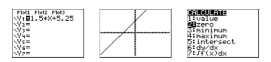
Graphing calculator solution: We should be able to ﬁnd the zero by sketching the graph of $f$ and noting where it crosses the $x$-axis. Start by loading the function $f(x)=1 .5x +5 .25$ into $\mathbf{Y1} $ in the Y= menu (see the ﬁrst image in Figure $\PageIndex{8}$).

Select 6:ZStandard from the ZOOM menu to produce the graph of $f$ (see the second image in Figure $\PageIndex{8}$). Press 2ND CALC to open the the CALCULATE menu (see the third image in Figure $\PageIndex{8}$). To ﬁnd the zero of the function $f$:

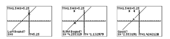
fig 5.3.8.png — Figure $\PageIndex{8}$: Finding the zero of $f(x)=1 .5x +5 .25$.

Select 2:zero from the CALCULATE menu. The calculator responds by asking for a “Left Bound?” (see the ﬁrst image in Figure $\PageIndex{9}$). Use the left arrow button to move the cursor so that it lies to the left of the $x$-intercept of $f$ and press ENTER.
The calculator responds by asking for a “Right Bound?” (see the second image in Figure $\PageIndex{9}$). Use the right arrow button to move the cursor so that it lies to the right of the $x$-intercept of $f$ and press ENTER.
The calculator responds by asking for a “Guess?” (see the third image in Figure $\PageIndex{9}$). As long as your cursor lies between the left- and right-bound marks at the top of the screen (see the third image in Figure $\PageIndex{9}$), you have a valid guess. Since the cursor already lies between the left- and right-bounds, simply press ENTER to use the current position of the cursor as your guess.

fig 5.3.9.png — Figure $\PageIndex{9}$: Using **2:zero** from the **CALCULATE** menu.

The calculator responds by approximating the zero of the function as shown in Figure $\PageIndex{10}$.

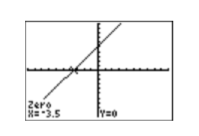
fig 5.3.10.png — Figure $\PageIndex{10}$: $−3.5$ is a zero off.

Note that the approximation found using the calculator agrees nicely with the zero found using the algebraic technique.

Exercise $\PageIndex{3}$

Find the zero(s) of the function $f(x)=2 .6x−9.62$.

Answer: $3.7$

Example $\PageIndex{4}$

How long will it take the projectile in Example $\PageIndex{2}$ to return to ground level?

Solution

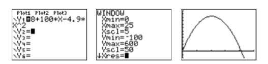
In Example $\PageIndex{2}$, the height of the projectile above the ground as a function of time is given by the equation \[y = 8 + 100t−4.9t^2 \nonumber \]When the projectile returns to the ground, its height above ground will be zero meters. To ﬁnd the time that this happens, substitute $y = 0$ in the last equation and solve for $t$. \[0 = 8 + 100t−4.9t^2 \nonumber \]Enter the equation $y = 8 + 100t − 4.9t^2$ into $\mathbf{Y1} $ in the Y= menu of your calculator (see the ﬁrst image in Figure $\PageIndex{11}$), then set the WINDOW parameters shown in the second image in Figure $\PageIndex{11}$. Push the GRAPH button to produce the graph of the function shown in the third image in Figure $\PageIndex{11}$.

fig 5.3.11.png — Figure $\PageIndex{11}$: Sketching the graph of $y = 8 + 100t−4.9t^2$.

In this example, the horizontal axis is actually the $t$-axis. So when we set $\mathrm{Xmin}$ and $\mathrm{Xmax}$, we’re actually setting bounds on the $t$-axis.

To ﬁnd the time when the projectile returns to ground level, we need to ﬁnd where the graph of $y = 8+100t−4.9t^2$ crosses the horizontal axis (in this case the t-axis) . Select 2:zero from the CALC menu. Use the arrow keys to move the cursor slightly to the left of the $t$-intercept, then press ENTER in response to “Left bound.” Move your cursor slightly to the right of the t-intercept, then press ENTER in response to “Right bound.” Leave your cursor where it is and press ENTER in response to “Guess.” The result is shown in Figure $\PageIndex{11}$.

Label the horizontal and vertical axes with $t$ and $y$, respectively (see Figure $\PageIndex{12}$). Include the units (seconds (s) and meters (m)).
Place your WINDOW parameters at the end of each axis (see Figure $\PageIndex{12}$).
Label the graph with its equation (see Figure $\PageIndex{12}$).
Draw a dashed vertical line through the $t$-intercept. Shade and label the $t$-value of the point where the dashed vertical line crosses the $t$-axis. This is the solution of the equation $0 = 8 + 100t−4.9t^2$ (see Figure $\PageIndex{12}$).

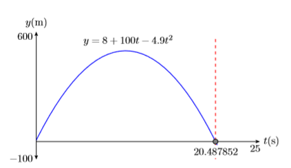
fig 5.3.12.png — Figure $\PageIndex{12}$: Reporting your graphical solution on your homework.

Rounding to the nearest tenth of a second, it takes the projectile approximately $t ≈ 20.5$ seconds to hit the ground.

Exercise $\PageIndex{4}$

If a projectile is launched with an initial velocity of $60$ meters per second from a rooftop $12$ meters above ground level, at what time will the projectile return to ground level?

Answer: $\approx 12.441734$ seconds

Search

Text Color

Text Size

Margin Size

Font Type