5.6: Multiplying Polynomials

Last updated
Save as PDF

Page ID: 19882

$ \newcommand{\vecs}[1]{\overset { \scriptstyle \rightharpoonup} {\mathbf{#1}} } $

$ \newcommand{\vecd}[1]{\overset{-\!-\!\rightharpoonup}{\vphantom{a}\smash {#1}}} $

$ \newcommand{\id}{\mathrm{id}}$ $ \newcommand{\Span}{\mathrm{span}}$

( \newcommand{\kernel}{\mathrm{null}\,}\) $ \newcommand{\range}{\mathrm{range}\,}$

$ \newcommand{\RealPart}{\mathrm{Re}}$ $ \newcommand{\ImaginaryPart}{\mathrm{Im}}$

$ \newcommand{\Argument}{\mathrm{Arg}}$ $ \newcommand{\norm}[1]{\| #1 \|}$

$ \newcommand{\inner}[2]{\langle #1, #2 \rangle}$

$ \newcommand{\Span}{\mathrm{span}}$

$ \newcommand{\id}{\mathrm{id}}$

$ \newcommand{\Span}{\mathrm{span}}$

$ \newcommand{\kernel}{\mathrm{null}\,}$

$ \newcommand{\range}{\mathrm{range}\,}$

$ \newcommand{\RealPart}{\mathrm{Re}}$

$ \newcommand{\ImaginaryPart}{\mathrm{Im}}$

$ \newcommand{\Argument}{\mathrm{Arg}}$

$ \newcommand{\norm}[1]{\| #1 \|}$

$ \newcommand{\inner}[2]{\langle #1, #2 \rangle}$

$ \newcommand{\Span}{\mathrm{span}}$ $ \newcommand{\AA}{\unicode[.8,0]{x212B}}$

$ \newcommand{\vectorA}[1]{\vec{#1}} % arrow$

$ \newcommand{\vectorAt}[1]{\vec{\text{#1}}} % arrow$

$ \newcommand{\vectorB}[1]{\overset { \scriptstyle \rightharpoonup} {\mathbf{#1}} } $

$ \newcommand{\vectorC}[1]{\textbf{#1}} $

$ \newcommand{\vectorD}[1]{\overrightarrow{#1}} $

$ \newcommand{\vectorDt}[1]{\overrightarrow{\text{#1}}} $

$ \newcommand{\vectE}[1]{\overset{-\!-\!\rightharpoonup}{\vphantom{a}\smash{\mathbf {#1}}}} $

$ \newcommand{\vecs}[1]{\overset { \scriptstyle \rightharpoonup} {\mathbf{#1}} } $

$ \newcommand{\vecd}[1]{\overset{-\!-\!\rightharpoonup}{\vphantom{a}\smash {#1}}} $

$\newcommand{\avec}{\mathbf a}$ $\newcommand{\bvec}{\mathbf b}$ $\newcommand{\cvec}{\mathbf c}$ $\newcommand{\dvec}{\mathbf d}$ $\newcommand{\dtil}{\widetilde{\mathbf d}}$ $\newcommand{\evec}{\mathbf e}$ $\newcommand{\fvec}{\mathbf f}$ $\newcommand{\nvec}{\mathbf n}$ $\newcommand{\pvec}{\mathbf p}$ $\newcommand{\qvec}{\mathbf q}$ $\newcommand{\svec}{\mathbf s}$ $\newcommand{\tvec}{\mathbf t}$ $\newcommand{\uvec}{\mathbf u}$ $\newcommand{\vvec}{\mathbf v}$ $\newcommand{\wvec}{\mathbf w}$ $\newcommand{\xvec}{\mathbf x}$ $\newcommand{\yvec}{\mathbf y}$ $\newcommand{\zvec}{\mathbf z}$ $\newcommand{\rvec}{\mathbf r}$ $\newcommand{\mvec}{\mathbf m}$ $\newcommand{\zerovec}{\mathbf 0}$ $\newcommand{\onevec}{\mathbf 1}$ $\newcommand{\real}{\mathbb R}$ $\newcommand{\twovec}[2]{\left[\begin{array}{r}#1 \\ #2 \end{array}\right]}$ $\newcommand{\ctwovec}[2]{\left[\begin{array}{c}#1 \\ #2 \end{array}\right]}$ $\newcommand{\threevec}[3]{\left[\begin{array}{r}#1 \\ #2 \\ #3 \end{array}\right]}$ $\newcommand{\cthreevec}[3]{\left[\begin{array}{c}#1 \\ #2 \\ #3 \end{array}\right]}$ $\newcommand{\fourvec}[4]{\left[\begin{array}{r}#1 \\ #2 \\ #3 \\ #4 \end{array}\right]}$ $\newcommand{\cfourvec}[4]{\left[\begin{array}{c}#1 \\ #2 \\ #3 \\ #4 \end{array}\right]}$ $\newcommand{\fivevec}[5]{\left[\begin{array}{r}#1 \\ #2 \\ #3 \\ #4 \\ #5 \\ \end{array}\right]}$ $\newcommand{\cfivevec}[5]{\left[\begin{array}{c}#1 \\ #2 \\ #3 \\ #4 \\ #5 \\ \end{array}\right]}$ $\newcommand{\mattwo}[4]{\left[\begin{array}{rr}#1 \amp #2 \\ #3 \amp #4 \\ \end{array}\right]}$ $\newcommand{\laspan}[1]{\text{Span}\{#1\}}$ $\newcommand{\bcal}{\cal B}$ $\newcommand{\ccal}{\cal C}$ $\newcommand{\scal}{\cal S}$ $\newcommand{\wcal}{\cal W}$ $\newcommand{\ecal}{\cal E}$ $\newcommand{\coords}[2]{\left\{#1\right\}_{#2}}$ $\newcommand{\gray}[1]{\color{gray}{#1}}$ $\newcommand{\lgray}[1]{\color{lightgray}{#1}}$ $\newcommand{\rank}{\operatorname{rank}}$ $\newcommand{\row}{\text{Row}}$ $\newcommand{\col}{\text{Col}}$ $\renewcommand{\row}{\text{Row}}$ $\newcommand{\nul}{\text{Nul}}$ $\newcommand{\var}{\text{Var}}$ $\newcommand{\corr}{\text{corr}}$ $\newcommand{\len}[1]{\left|#1\right|}$ $\newcommand{\bbar}{\overline{\bvec}}$ $\newcommand{\bhat}{\widehat{\bvec}}$ $\newcommand{\bperp}{\bvec^\perp}$ $\newcommand{\xhat}{\widehat{\xvec}}$ $\newcommand{\vhat}{\widehat{\vvec}}$ $\newcommand{\uhat}{\widehat{\uvec}}$ $\newcommand{\what}{\widehat{\wvec}}$ $\newcommand{\Sighat}{\widehat{\Sigma}}$ $\newcommand{\lt}{<}$ $\newcommand{\gt}{>}$ $\newcommand{\amp}{&}$ $\definecolor{fillinmathshade}{gray}{0.9}$

In this section we will find the products of polynomial expressions and functions. We start with the product of two monomials, then graduate to the product of a monomial and polynomial, and complete the study by finding the product of any two polynomials.

The Product of Monomials

As long as all of the operations are multiplication, we can use the commutative and associative properties to change the order and regroup.

Example $\PageIndex{1}$

Multiply: $−5(7y)$. Simplify: $−5(7y)$.

Solution

Use the commutative and associative properties to change the order and regroup.

\[\begin{align*} -5(7 y) &= [(-5)(7)] y \quad &\color {Red} \text { Reorder. Regroup. } \\ &= -35 y \quad &\color {Red} \text { Multiply: } (-5)(7)=-35 \end{align*} \nonumber \]

Exercise $\PageIndex{1}$

Multiply: $3(4 x)$

Answer: $12x$

Example $\PageIndex{2}$

Multiply: $(−3x^2)(4x^3)$. Simplify: $(−3x^2)(4x^3)$.

Solution

Use the commutative and associative properties to change the order and regroup.

\[\begin{aligned} \left(-3 x^{2}\right)\left(4 x^{3}\right) &= [(-3)(4)]\left(x^{2} x^{3}\right) \quad \color {Red} \text { Reorder. Regroup. } \\ &= -12 x^{5} \quad \color {Red} \text { Multiply: }(-3)(4)=12, x^{2} x^{3}=x^{5}\end{aligned} \nonumber\]

Exercise $\PageIndex{2}$

Multiply: $(7 y^5)(−2y^2)$

Answer: $-14 y^{7}$

Example $\PageIndex{3}$

Multiply: $(−2a^2b^3)(−5a^3b)$. Simplify: $(−2a^2b^3)(−5a^3b)$.

Solution

Use the commutative and associative properties to change the order and regroup.

\[\begin{aligned} \left(-2 a^{2} b^{3}\right)\left(-5 a^{3} b\right) &=[(-2)(-5)]\left(a^{2} a^{3}\right)\left(b^{3} b\right) \quad \color {Red} \text { Reorder. Regroup. } \\ &=10 a^{5} b^{4} \quad \color {Red} \text { Multiply: }(-2)(-5)=10, a^{2} a^{3}=a^{5}, \text { and } b^{3} b=b^{4}\end{aligned} \nonumber\]

Exercise $\PageIndex{3}$

Multiply: $( −6st^2)(3s^3t^4)$

Answer: $-18 s^{4} t^{6}$

When multiplying monomials, it is much more efficient to make the required calculations mentally. In the case of Example $\PageIndex{1}$, multiply $−5$ and $7$ mentally to get\[−5(7y)=−35y \nonumber \]In the case of Example $\PageIndex{2}$, multiply $−3$ and $4$ to get $−12$, then repeat the base $x$ and add exponents to get\[(−3x^2)(4x^3)=−12x^5 \nonumber \]Finally, in the case of Example $\PageIndex{3}$, multiply $−2$ and $−5$ to get $10$, then repeat the bases and add their exponents.\[(−2a^2b^3)(−5a^3b) = 10 a^5b^4 \nonumber \]

Multiplying a Monomial and a Polynomial

Now we turn our attention to the product of a monomial and a polynomial.

Example $\PageIndex{4}$

Multiply: $5\left(3 x^{2}-4 x-8\right)$

Solution

We need to first distribute the $5$ times each term of the polynomial. Then we multiply the resulting monomials mentally.

\[\begin{aligned} 5\left(3 x^{2}-4 x-8\right) &=5\left(3 x^{2}\right)-5(4 x)-5(8) \\ &=15 x^{2}-20 x-40 \end{aligned} \nonumber \]

Exercise $\PageIndex{4}$

Multiply: $4\left(-2 y^{2}+3 y+5\right)$

Answer: $-8 y^{2}+12 y+20$

Example $\PageIndex{5}$

Multiply: $2 y(-3 y+5) $

Solution

We need to first distribute the $2y$ times each term of the polynomial. Then we multiply the resulting monomials mentally.

\[\begin{aligned} 2 y(-3 y+5) &=2 y(-3 y)+2 y(5) \\ &=-6 y^{2}+10 y \end{aligned} \nonumber \]

Exercise $\PageIndex{5}$

Multiply: $-3 x(4-2 x)$

Answer: $-12 x+6 x^{2}$

Example $\PageIndex{6}$

Multiply: $-3 a b\left(a^{2}+2 a b-b^{2}\right)$

Solution

We need to first distribute the $−3ab$ times each term of the polynomial. Then we multiply the resulting monomials mentally.

\[\begin{aligned}-3 a b\left(a^{2}+2 a b-b^{2}\right) &=-3 a b\left(a^{2}\right)+(-3 a b)(2 a b)-(-3 a b)\left(b^{2}\right) \\ &=-3 a^{3} b+\left(-6 a^{2} b^{2}\right)-\left(-3 a b^{3}\right) \\ &=-3 a^{3} b-6 a^{2} b^{2}+3 a b^{3} \end{aligned} \nonumber \]

Alternate solution:

It is far more efficient to perform most of the steps of the product $−3ab(a^2 +2ab−b^2)$ mentally. We know we must multiply $−3ab$ times each of the terms of the polynomial $a^2 +2ab−b^2$. Here are our mental calculations:

$−3ab$ times $a^2$ equals $−3a3b$.
$−3ab$ times $2ab$ equals $−6a^2b^2$.
$−3ab$ times $−b^2$ equals $3ab^3$.

Thinking in this manner allows us to write down the answer without any of the steps shown in our first solution. That is, we immediately write:

\[-3 a b\left(a^{2}+2 a b-b^{2}\right)=-3 a^{3} b-6 a^{2} b^{2}+3 a b^{3} \nonumber \]

Exercise $\PageIndex{6}$

Multiply: $2 x y\left(x^{2}-4 x y^{2}+7 x\right)$

Answer: $2 x^{3} y-8 x^{2} y^{3}+14 x^{2} y$

Example $\PageIndex{7}$

Multiply: $-2 z^{2}\left(z^{3}+4 z^{2}-11\right)$

Solution

We need to first distribute the $−2z^2$ times each term of the polynomial. Then we multiply the resulting monomials mentally.

\[\begin{aligned}-2 z^{2}\left(z^{3}+4 z^{2}-11\right) &=-2 z^{2}\left(z^{3}\right)+\left(-2 z^{2}\right)\left(4 z^{2}\right)-\left(-2 z^{2}\right)(11) \\ &=-2 z^{5}+\left(-8 z^{4}\right)-\left(-22 z^{2}\right) \\ &=-2 z^{5}-8 z^{4}+22 z^{2} \end{aligned} \nonumber \]

Alternate solution:

It is far more efficient to perform most of the steps of the product $−2z^2(z^3 +4z^2 −11)$ mentally. We know we must multiply $−2z^2$ times each of the terms of the polynomial $z^3 +4z^2 −11$. Here are our mental calculations:

$−2z^2$ times $z^3$ equals $−2z^5$.
$−2z^2$ times $4z^2$ equals $−8z^4$.
$−2z^2$ times $−11$ equals $22z^2$.

Thinking in this manner allows us to write down the answer without any of the steps shown in our first solution. That is, we immediately write:

\[-2 z^{2}\left(z^{3}+4 z^{2}-11\right)=-2 z^{5}-8 z^{4}+22 z^{2} \nonumber \]

Exercise $\PageIndex{7}$

Multiply: $-5 y^{3}\left(y^{2}-2 y+1\right)$

Answer: $-5 y^{5}+10 y^{4}-5 y^{3}$

Multiplying Polynomials

Now that we’ve learned how to take the product of two monomials or the product of a monomial and a polynomial, we can apply what we’ve learned to multiply two arbitrary polynomials.

Before we begin with the examples, let’s revisit the distributive property. We know that\[2 \cdot(3+4)=2 \cdot 3+2 \cdot 4 \nonumber \]Both sides are equal to $14$. We’re used to having the monomial factor on the left, but it can also appear on the right.\[(3+4) \cdot 2=3 \cdot 2+4 \cdot 2 \nonumber \]Again, both sides equal $14$. So, whether the monomial appears on the left or right makes no difference; that is, $a(b + c)=ab + ac$ and $(b + c)a = ba + ca$ give the same result. In each case, you multiply $a$ times both terms of $b + c$.

Example $\PageIndex{8}$

Multiply: $(2x + 5)(3x + 2)$

Solution

Note that $(2x + 5)(3x + 2)$ has the form $(b + c)a$, where $a$ is the binomial $3x+2$. Because $(b+c){\color {Red}a} = b{\color {Red}a}+c{\color {Red}a}$, we will multiply $3x+2$ times both terms of $2x + 5$ in the following manner.

\[(2x + 5){\color {Red}(3x + 2)}=2x{\color {Red}(3x + 2)}+5{\color {Red}(3x + 2)} \nonumber \]

Now we distribute monomials times polynomials, then combine like terms.

\[\begin{array}{l}{=6 x^{2}+4 x+15 x+10} \\ {=6 x^{2}+19 x+10}\end{array} \nonumber \]

Thus, $(2 x+5)(3 x+2)=6 x^{2}+19 x+10$

Exercise $\PageIndex{8}$

Multiply: $(3x + 4)(5x + 1)$

Answer: $15 x^{2}+23 x+4$

Example $\PageIndex{9}$

Multiply: $(x+5)\left(x^{2}+2 x+7\right)$

Solution

Note that $(x+5)(x^2 +2x+7)$ has the form $(b+c)a$, where $a$ is the trinomial $x^2 +2x+7$. Because $(b+c){\color {Red}a} = b{\color {Red}a}+c{\color {Red}a}$, we will multiply $x^2 +2x+7$ times both terms of $x + 5$ in the following manner.

\[(x+5){\color {Red}\left(x^{2}+2 x+7\right)}=x{\color {Red}\left(x^{2}+2 x+7\right)}+5{\color {Red}\left(x^{2}+2 x+7\right)} \nonumber \]

Now we distribute monomials times polynomials, then combine like terms.

\[\begin{array}{l}{=x^{3}+2 x^{2}+7 x+5 x^{2}+10 x+35} \\ {=x^{3}+7 x^{2}+17 x+35}\end{array} \nonumber \]

Thus, $(x+5)\left(x^{2}+2 x+7\right)=x^{3}+7 x^{2}+17 x+35$

Exercise $\PageIndex{9}$

Multiply: $(z+4)\left(z^{2}+3 z+9\right)$

Answer: $z^{3}+7 z^{2}+21 z+36$

Speeding Things Up a Bit

Let’s re-examine Example $\PageIndex{9}$ with the hope of unearthing a pattern that will allow multiplication of polynomials to proceed more quickly with less work. Note the first step of Example $\PageIndex{9}$.

\[(x+5){\color {Red}\left(x^{2}+2 x+7\right)}=x{\color {Red}\left(x^{2}+2 x+7\right)}+5{\color {Red}\left(x^{2}+2 x+7\right)} \nonumber \]

Note that the first product on the right is the result of taking the product of the first term of $x + 5$ and $x^2 +2x + 7$. Similarly, the second product on the right is the result of taking the product of the second term of $x + 5$ and $x^2 +2x + 7$. Next, let’s examine the result of the second step.

\[(x+5)\left(x^{2}+2 x+7\right)=x^{3}+2 x^{2}+7 x+5 x^{2}+10 x+35 \nonumber \]

The first three terms on the right are the result of multiplying $x$ times $x^2+2x+7$.

$fig 5.6.a.png$

The second set of three terms on the right are the result of multiplying $5$ times $x^2 +2x + 7$.

$fig 5.6.b.png$

These notes suggest an efficient shortcut. To multiply $x+5$ times $x^2 +2x+7$,

Multiply $x$ times each term of $x^2 +2x + 7$.
Multiply $5$ times each term of $x^2 +2x + 7$.
Combine like terms.

This process would have the following appearance.

\[\begin{aligned}(x+5)\left(x^{2}+2 x+7\right) &=x^{3}+2 x^{2}+7 x+5 x^{2}+10 x+35 \\ &=x^{3}+7 x^{2}+17 x+35 \end{aligned} \nonumber \]

Example $\PageIndex{10}$

Use the shortcut technique described above to simplify: $(2 y-6)\left(3 y^{2}+4 y+11\right)$

Solution

Multiply $2y$ times each term of $3y^2 +4 y + 11$, then multiply $−6$ times each term of $3y^2 +4y + 11$. Finally, combine like terms.

\[\begin{aligned}(2 y-6)\left(3 y^{2}+4 y+11\right) &=6 y^{3}+8 y^{2}+22 y-18 y^{2}-24 y-66 \\ &=6 y^{3}-10 y^{2}-2 y-66 \end{aligned} \nonumber \]

Exercise $\PageIndex{10}$

Multiply: $(3 x+2)\left(4 x^{2}-x+10\right)$

Answer: $12 x^{3}+5 x^{2}+28 x+20$

Example $\PageIndex{11}$

Use the shortcut technique to simplify $(a+b)^{2}$

Solution

To simplify $(a+b)^2$, we first must write $a+b$ as a factor two times.

\[(a+b)^{2}=(a+b)(a+b) \nonumber \]

Next, multiply a times both terms of $a + b$, multiply b times both terms of $a + b$, then combine like terms.

\[\begin{array}{l}{=a^{2}+a b+b a+b^{2}} \\ {=a^{2}+2 a b+b^{2}}\end{array} \nonumber \]

Note that $ab = ba$ because multiplication is commutative, so $ab + ba =2ab$.

Exercise $\PageIndex{11}$

Multiply: $(3 y-2)^{2}$

Answer: $9 y^{2}-12 y+4$

Example $\PageIndex{12}$

Use the shortcut technique to simplify: $\left(x^{2}+x+1\right)\left(x^{2}-x-1\right)$

Solution

This time the first factor contains three terms, $x^2$, $x$, and $1$, so we first multiply $x^2$ times each term of $x^2 −x−1$, then $x$ times each term of $x^2 −x−1$, and $1$ times each term of $x^2 −x−1$. Then we combine like terms.

\[\begin{aligned}\left(x^{2}+x+1\right)\left(x^{2}-x-1\right) &=x^{4}-x^{3}-x^{2}+x^{3}-x^{2}-x+x^{2}-x-1 \\ &=x^{4}-x^{2}-2 x-1 \end{aligned} \nonumber \]

Exercise $\PageIndex{12}$

Multiply: $\left(a^{2}-2 a+3\right)\left(a^{2}+2 a-3\right)$

Answer: $a^{4}-4 a^{2}+12 a-9$

Some Applications

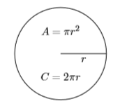
Recall that the area of a circle of radius $r$ is found using the formula $A = πr^2$. The circumference (distance around) of a circle of radius $r$ is found using the formula $C =2πr$ (see Figure $\PageIndex{1}$).

fig 5.6.1.png — Figure $\PageIndex{1}$: Formulae for the area and circumference of a circle of radius $r$.

Example $\PageIndex{13}$

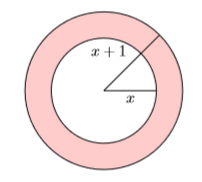
In Figure $\PageIndex{2}$ are pictured two concentric circles (same center).The inner circle has radius $x$ and the outer circle has radius $x + 1$. Find the area of the shaded region (called an annulus) as a function of $x$.

fig 5.6.2.png — Figure $\PageIndex{2}$: Find the area of the shaded region.

Solution

We can find the area of the shaded region by subtracting the area of the inner circle from the area of the outer circle.

\[A=\text { Area of outer circle - Area of inner circle} \nonumber \]

We use the formula $A = πr^2$ to compute the area of each circle. Because the outer circle has radius $x+1$, it has area $π(x+1)^2$. Because the inner circle has radius $x$, it has area $πx^2$.

\[=\pi(x+1)^{2}-\pi x^{2} \nonumber \]

Next, we’ll expand $(x + 1)^2$, then combine like terms.

\[\begin{array}{l}{=\pi(x+1)(x+1)-\pi x^{2}} \\ {=\pi\left(x^{2}+x+x+1\right)-\pi x^{2}} \\ {=\pi\left(x^{2}+2 x+1\right)-\pi x^{2}}\end{array} \nonumber \]

Finally, distribute $π$ times each term of $x^2 +2x + 1$, then combine like terms.

\[\begin{array}{l}{=\pi x^{2}+2 \pi x+\pi-\pi x^{2}} \\ {=2 \pi x+\pi}\end{array} \nonumber \]

Hence, the area of the shaded region is $A =2πx+ π$.

Exercise $\PageIndex{13}$

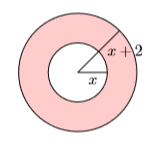
Two concentric circles are shown below. The inner circle has radius $x$ and the outer circle has radius $x + 2$. Find the area of the shaded region as a function of $x$.

$Ex 5.6.13.png$

Answer: $4 \pi x+4 \pi$

Example $\PageIndex{14}$

The demand for widgets is a function of the unit price, where the demand is the number of widgets the public will buy and the unit price is the amount charged for a single widget. Suppose that the demand is given by the function $x = 270−0.75p$, where $x$ is the demand and $p$ is the unit price. Note how the demand decreases as the unit price goes up (makes sense). Use the graphing calculator to determine the unit price a retailer should charge for widgets so that his revenue from sales equals $\$20,000$.

Solution

To determine the revenue $(R)$, you multiply the number of widgets sold $(x)$ by the unit price $(p)$.

\[R=xp \label {Eq5.6.1} \]

However, we know that the number of units sold is the demand, given by the formula

\[x = 270−0.75p \label {Eq5.6.2} \]

Substitute equation $\ref {Eq5.6.2}$ into equation $\ref {Eq5.6.1}$ to obtain the revenue as a function of the unit price.

\[R = (270−0.75p)p \nonumber \]

Expand.

\[R=270 p-0.75 p^{2} \label {Eq5.6.3} \]

We’re asked to determine the unit price that brings in a revenue of $\$20,000$. Substitute $\$20,000$ for $R$ in equation $\ref {Eq5.6.3}$.

\[20000=270 p-0.75 p^{2} \label {Eq5.6.4} \]

Enter each side of equation $\ref {Eq5.6.4}$ into the Y= menu of your calculator (see the first image in Figure $\PageIndex{3}$). After some experimentation, we settled on the WINDOW parameters shown in the second image of Figure $\PageIndex{3}$. After making these settings, push the GRAPH button to produce the graph shown in the third image in Figure $\PageIndex{3}$.

fig 5.6.3.png — Figure $\PageIndex{3}$: Solving $20000 = 270p−0.75p^2$.

Note that the third image in Figure $\PageIndex{3}$ shows that there are two solutions, that is, two ways we can set the unit price to obtain a revenue of $\$20,000$. To find the first solution, select 5:intersect from the CALC menu, press ENTER in response to “First curve,” press ENTER in response to “Second curve,” then move your cursor closer to the point of intersection on the left and press ENTER in response to “Guess.” The result is shown in the first image in Figure $\PageIndex{4}$.

Repeat the process to find the second point of intersection. The result is shown in the second image in Figure $\PageIndex{4}$.

fig 5.6.4.png — Figure $\PageIndex{4}$: Finding the points of intersection.

Note

In this example, the horizontal axis is actually the $p$-axis. So when we set $\mathrm{Xmin}$ and $\mathrm{Xmax}$, we’re actually setting bounds on the $p$-axis.

Reporting the solution on your homework:

fig 5.6.5.png — Figure $\PageIndex{5}$: Reporting your graphical solution on your homework.

Duplicate the image in your calculator’s viewing window on your homework page. Use a ruler to draw all lines, but freehand any curves.

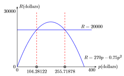
Label the horizontal and vertical axes with $p$ and $R$, respectively (see Figure $\PageIndex{5}$). Include the units (dollars and dollars).
Place your WINDOW parameters at the end of each axis (see Figure $\PageIndex{5}$).
Label each graph with its equation (see Figure $\PageIndex{5}$).
Drop a dashed vertical line through each point of intersection. Shade and label the $p$-values of the points where the dashed vertical lines cross the $p$-axis. These are the solutions of the equation $20000 = 270p− 0.75p^2$ (see Figure $\PageIndex{5}$).

Rounding to the nearest penny, setting the unit price at either $\$104.28$ or $\$255.72$ will bring in a revenue of $\$20,000$.

Exercise $\PageIndex{14}$

Suppose that the demand for gadgets is given by the function $x = 320−1.5p$, where $x$ is the demand and $p$ is the unit price. Use the graphing calculator to determine the unit price a retailer should charge for gadgets so that her revenue from sales equals $\$12,000$.

Answer: $\$ 48.55$ or $\$ 164.79$

Search

Text Color

Text Size

Margin Size

Font Type