7.7: Solving Rational Equations

When simplifying complex fractions in the previous section, we saw that multiplying both numerator and denominator by the appropriate expression could “clear” all fractions from the numerator and denominator, greatly simplifying the rational expression.

In this section, a similar technique is used.

Clear the Fractions from a Rational Equation

If your equation has rational expressions, multiply both sides of the equation by the least common denominator to clear the equation of rational expressions.

Let’s look at an example.

Example \(\PageIndex{1}\)

Solve the following equation for x.

\[\frac{x}{2}-\frac{2}{3}=\frac{3}{4} \nonumber \]

Solution

To clear this equation of fractions, we will multiply both sides by the common denominator for 2, 3, and 4, which is 12. Distribute 12 in the second step.

\[\begin{aligned} \color{blue}{12}\left(\frac{x}{2}-\frac{2}{3}\right) &=\left(\frac{3}{4}\right) \color{blue}{12} \\ \color{blue}{12}\left(\frac{x}{2}\right)-\color{blue}{12}\left(\frac{2}{3}\right) &=\left(\frac{3}{4}\right) \color{blue}{12} \end{aligned} \nonumber \]

Multiply.

\[6 x-8=9 \nonumber \]

We’ve succeeded in clearing the rational expressions from the equation by multiplying through by the common denominator. We now have a simple linear equation which can be solved by first adding 8 to both sides of the equation, followed by dividing both sides of the equation by 6.

\[\begin{aligned} 6 x &=17 \\ x &=\frac{17}{6} \end{aligned} \nonumber \]

We’ll leave it to our readers to check this solution.

Let’s try another example.

Example \(\PageIndex{2}\)

Solve the following equation for x. \[6=\frac{5}{x}+\frac{6}{x^{2}} \nonumber \]

Solution

In this equation, the denominators are 1, x, and \(x^2\), and the common denominator for both sides of the equation is \(x^2\). Consequently, we begin the solution by first multiplying both sides of the equation by \(x^2\).

\[\begin{array}{l}{\color{blue}{x^{2}}(6)=\left(\frac{5}{x}+\frac{6}{x^{2}}\right) \color{blue}{x^{2}}} \\ {\color{blue}{x^{2}}(6)=\left(\frac{5}{x}\right) \color{blue}{x^{2}}+\left(\frac{6}{x^{2}}\right) \color{blue}{x^{2}}}\end{array} \nonumber \]

Simplify.

\[6 x^{2}=5 x+6 \nonumber \]

Note that multiplying both sides of the original equation by the least common denominator clears the equation of all rational expressions. This last equation is nonlinear, so make one side of the equation equal to zero by subtracting 5x and 6 from both sides of the equation.

\[6 x^{2}-5 x-6=0 \nonumber \]

To factor the left-hand side of this equation, note that it is a quadratic trinomial with ac = (6)(−6) = −36. The integer pair 4 and −9 have product −36 and sum −5. Split the middle term using this pair and factor by grouping.

\[\begin{aligned} 6 x^{2}+4 x-9 x-6 &=0 \\ 2 x(3 x+2)-3(3 x+2) &=0 \\(2 x-3)(3 x+2) &=0 \end{aligned} \nonumber \]

The zero product property forces either

\[2 x-3=0 \quad \text { or } \quad 3 x+2=0 \nonumber \]

Each of these linear equations is easily solved.

\[x=\frac{3}{2} \quad \text { or } \quad x=-\frac{2}{3} \nonumber \]

Of course, we should always check our solutions. Substituting x = 3/2 into the right-hand side of the original equation (4),

\[\frac{5}{x}+\frac{6}{x^{2}}=\frac{5}{3 / 2}+\frac{6}{(3 / 2)^{2}}=\frac{5}{3 / 2}+\frac{6}{9 / 4} \nonumber \]

In the final expression, multiply top and bottom of the first fraction by 2, top and bottom of the second fraction by 4.

\[\frac{5}{3 / 2} \cdot \color{blue}{\frac{2}{2}}+\frac{6}{9 / 4} \cdot \color{blue}{\frac{4}{4}}=\frac{10}{3}+\frac{24}{9} \nonumber \]

Make equivalent fractions with a common denominator of 9 and add.

\[\frac{10}{3} \cdot \color{blue}{\frac{3}{3}}+\frac{24}{9}=\frac{30}{9}+\frac{24}{9}=\frac{54}{9}=6 \nonumber \]

Note that this result is identical to the left-hand side of the original equation (4). Thus, x = 3/2 checks.

This example clearly demonstrates that the check can be as difficult and as time consuming as the computation used to originally solve the equation. For this reason, we tend to get lazy and not check our answers as we should. There is help, however, as the graphing calculator can help us check the solutions of equations.

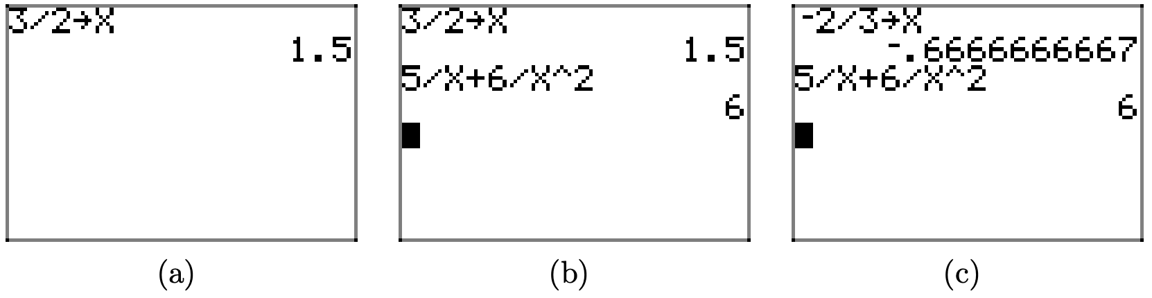
First, enter the solution 3/2 in your calculator screen, push the STOI button, then push the X button, and execute the resulting command on the screen by pushing the ENTER key. The result is shown in Figure \(\PageIndex{1}\)(a).

Next, enter the expression 5/X+6/Xˆ2 and execute the resulting command on the screen by pushing the ENTER key. The result is shown in Figure \(\PageIndex{1}\)(b). Note that the result is 6, the same as computed by hand above, and it matches the left-hand side of the original equation (4). We’ve also used the calculator to check the second solution x = −2/3. This is shown in Figure \(\PageIndex{4}\)(c).

Figure \(\PageIndex{1}\). Using the graphing calculator to check the solutions of equation (4).

Let’s look at another example.

Example \(\PageIndex{3}\)

Solve the following equation for x.

\[\frac{2}{x^{2}}=1-\frac{2}{x} \nonumber \]

Solution

First, multiply both sides of equation (6) by the common denominator \(x^2\).

\[\begin{aligned} \color{blue}{x^{2}}\left(\frac{2}{x^{2}}\right) &=\left(1-\frac{2}{x}\right) \color{blue}{x^{2}} \\ 2 &=x^{2}-2 x \end{aligned} \nonumber \]

Make one side zero.

\[0=x^{2}-2 x-2 \nonumber \]

The right-hand side is a quadratic trinomial with ac = (1)(−2) = −2. There are no integer pairs with product −2 that sum to −2, so this quadratic trinomial does not factor. Fortunately, the equation is quadratic (second degree), so we can use the quadratic formula with a = 1, b = −2, and c = −2.

\[x=\frac{-b \pm \sqrt{b^{2}-4 a c}}{2 a}=\frac{-(-2) \pm \sqrt{(-2)^{2}-4(1)(-2)}}{2(1)}=\frac{2 \pm \sqrt{12}}{2} \nonumber \]

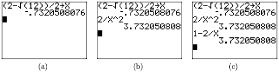
This gives us two solutions, \(x=(2-\sqrt{12}) / 2\) and \(x=(2+\sqrt{12}) / 2\). Let’s check the solution \(x=(2-\sqrt{12}) / 2\). First, enter this result in your calculator, press the STOI button, press X, then press the ENTER key to execute the command and store the solution in the variable X. This command is shown in Figure \(\PageIndex{2}\)(a).

Enter the left-hand side of the original equation (6) as 2/xˆ2 and press the ENTER key to execute this command. This is shown in Figure \(\PageIndex{2}\)(b).

Enter the right-hand side of the original equation (6) as 1-2/X and press the ENTER key to execute this command. This is shown in Figure \(\PageIndex{2}\)(c). Note that the left- and right-hand sides of equation (6) are both shown to equal 3.732050808 at \(x=(2-\sqrt{12}) / 2\) (at X = -0.7320508076), as shown in Figure \(\PageIndex{2}\)(c). This shows that \(x=(2-\sqrt{12}) / 2\) is a solution of equation (6).

We leave it to our readers to check the second solution, \(x=(2+\sqrt{12}) / 2\).

Figure \(\PageIndex{2}\). Using the graphing calculator to check the solutions of equation (6).

Let’s look at another example, this one involving function notation.

Example \(\PageIndex{4}\)

Consider the function defined by \[f(x)=\frac{1}{x}+\frac{1}{x-4} \nonumber \] Solve the equation f(x) = 2 for x using both graphical and analytical techniques, then compare solutions. Perform each of the following tasks.

a. Sketch the graph of f on graph paper. Label the zeros of f with their coordinates and the asymptotes of f with their equations.

b. Add the graph of y = 2 to your plot and estimate the coordinates of where the graph of f intersects the graph of y = 2.

c. Use the intersect utility on your calculator to find better approximations of the points where the graphs of f and y = 2 intersect.

d. Solve the equation f(x) = 2 algebraically and compare your solutions to those found in part (c).

Solution

For the graph in part (a), we need to find the zeros of f and the equations of any vertical or horizontal asymptotes.

To find the zero of the function f, we find a common denominator and add the two rational expressions in equation (8).

\[f(x)=\frac{1}{x}+\frac{1}{x-4}=\frac{x-4}{x(x-4)}+\frac{x}{x(x-4)}=\frac{2 x-4}{x(x-4)} \nonumber \]

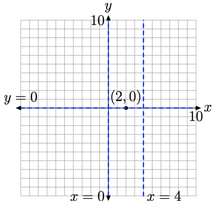
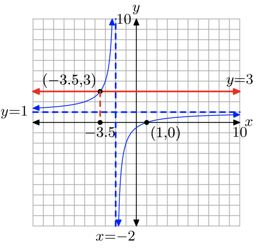
Note that the numerator of this result equal zero (but not the denominator) when x = 2. This is the zero of f. Thus, the graph of f has x-intercept at (2, 0), as shown in Figure \(\PageIndex{4}\).

Note that the rational function in equation (9) is reduced to lowest terms. The denominators of x and x + 4 in equation (9) are zero when x = 0 and x = 4. These are our vertical asymptotes, as shown in Figure \(\PageIndex{4}\).

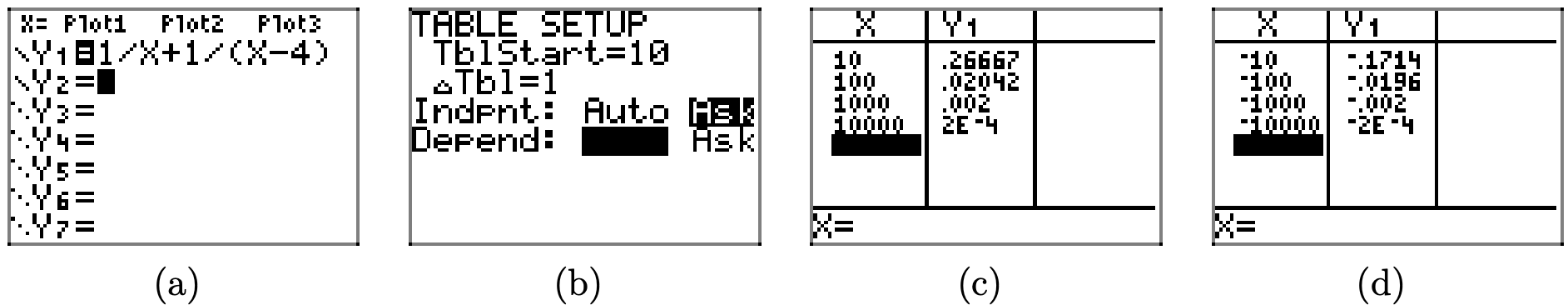
To find the horizontal asymptotes, we need to examine what happens to the function values as x increases (or decreases) without bound. Enter the function in the Y= menu with 1/X+1/(X-4), as shown in Figure \(\PageIndex{3}\)(a). Press 2nd TBLSET, then highlight ASK for the independent variable and press ENTER to make this selection permanent, as shown in Figure \(\PageIndex{3}\)(b).

Press 2nd TABLE, then enter 10, 100, 1,000, and 10,000, as shown in Figure \(\PageIndex{3}\)(c). Note how the values of Y1 approach zero. In Figure \(\PageIndex{3}\)(d), as x decreases without bound, the end-behavior is the same. This is an indication of a horizontal asymptote at y = 0, as shown in Figure \(\PageIndex{4}\).

Figure \(\PageIndex{3}\). Examining the end-behavior of f with the graphing calculator.

Figure \(\PageIndex{4}\). Placing the horizontal and vertical asymptotes and the x-intercept of the graph of the function f.

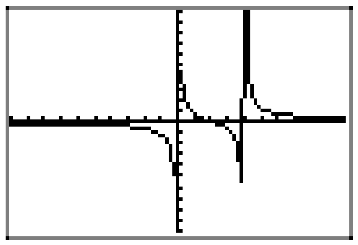
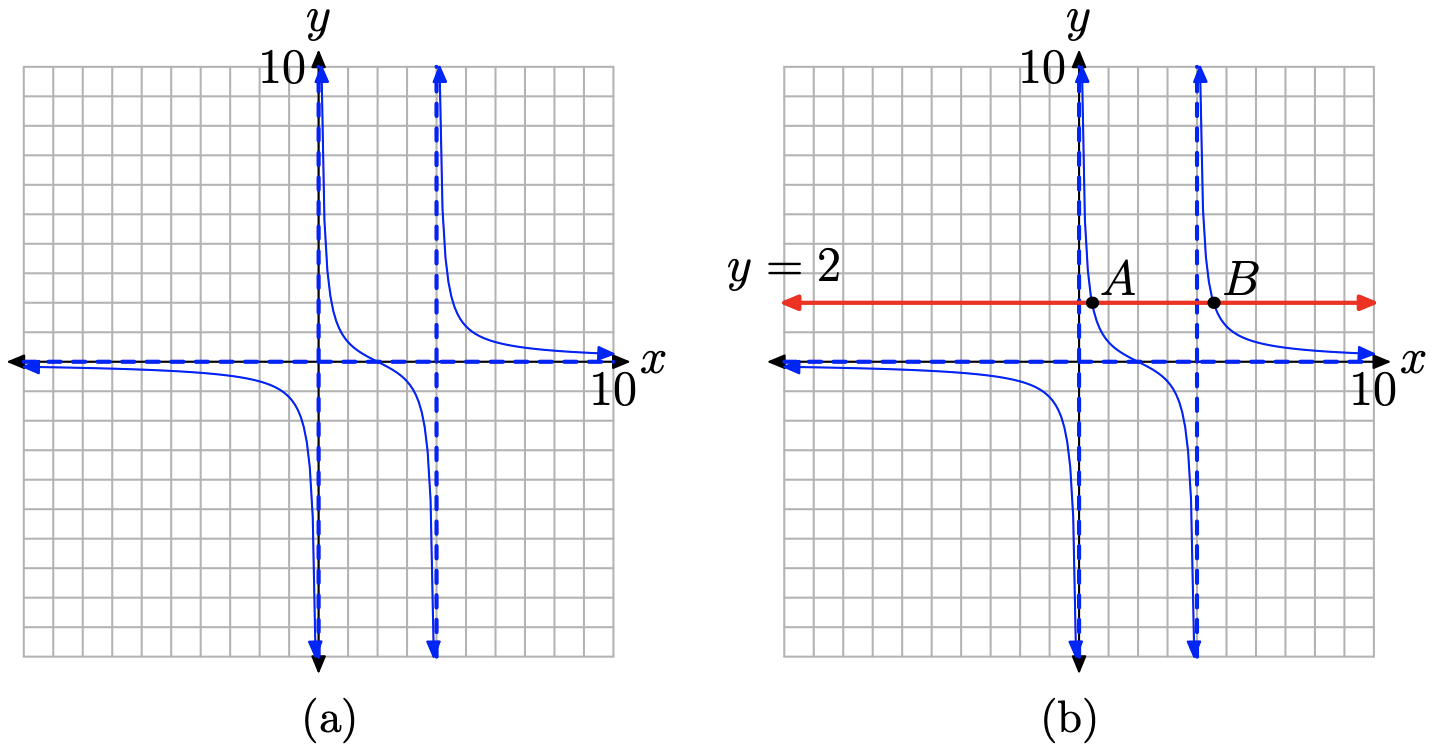
At this point, we already have our function f loaded in Y1, so we can press the ZOOM button and select 6:ZStandard to produce the graph shown in Figure \(\PageIndex{5}\). As expected, the graphing calculator does not do a very good job with the rational function f, particularly near the discontinuities at the vertical asymptotes. However, there is enough information in Figure \(\PageIndex{5}\), couple with our advanced work summarized in Figure \(\PageIndex{4}\), to draw a very nice graph of the rational function on our graph paper, as shown in Figure \(\PageIndex{6}\)(a). Note: We haven’t labeled asymptotes with equations, nor zeros with coordinates, in Figure \(\PageIndex{6}\)(a), as we thought the picture might be a little crowded. However, you should label each of these parts on your graph paper, as we did in Figure \(\PageIndex{4}\).

Figure \(\PageIndex{5}\). The graph of f as drawn on the calculator.

Let’s now address part (b) by adding the horizontal line y = 2 to the graph, as shown in Figure \(\PageIndex{6}\)(b). Note that the graph of y = 2 intersects the graph of the rational function f at two points A and B. The x-values of points A and B are the solutions to our equation f(x) = 2.

We can get a crude estimate of the x-coordinates of points A and B right off our graph paper. The x-value of point A is approximately \(x \approx 0.3\), while the x-value of point B appears to be approximately \(x \approx 4.6\).

Figure \(\PageIndex{6}\). Solving f(x) = 2 graphically.

Next, let’s address the task required in part (c). We have very reasonable estimates of the solutions of f(x) = 2 based on the data presented in Figure \(\PageIndex{6}\)(b). Let’s use the graphing calculator to improve upon these estimates.

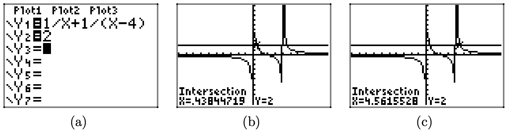
First, load the equation Y2=2 into the Y= menu, as shown in Figure \(\PageIndex{7}\)(a). We need to find where the graph of Y1 intersects the graph of Y2, so we press 2nd CALC and select 5:intersect from the menu. In the usual manner, select “First curve,” “Second curve,” and move the cursor close to the point you wish to estimate. This is your “Guess.” Perform similar tasks for the second point of intersection.

Our results are shown in Figures \(\PageIndex{7}\)(b) and Figures \(\PageIndex{7}\)(c). The estimate in Figure \(\PageIndex{7}\)(b) has \(x \approx 0.43844719\), while that in Figure \(\PageIndex{7}\)(c) has \(x \approx 4.5615528\). Note that these are more accurate than the approximations of \(x \approx 0.3\) and \(x \approx 4.6\) captured from our hand drawn image in Figure \(\PageIndex{6}\)(b).

Figure \(\PageIndex{7}\). Solving f(x) = 2 graphically.

Finally, let’s address the request for an algebraic solution of f(x) = 2 in part (d). First, replace f(x) with 1/x + 1/(x − 4) to obtain

\[\begin{aligned} f(x) &=2 \\ \frac{1}{x}+\frac{1}{x-4} &=2 \end{aligned} \nonumber \]

Multiply both sides of this equation by the common denominator x(x − 4).

\[\begin{aligned} \color{blue}{x(x-4)}\left[\frac{1}{x}+\frac{1}{x-4}\right] &=[2] \color{blue}{x(x-4)} \\ \color{blue}{x(x-4)}\left[\frac{1}{x}\right]+\color{blue}{x(x-4)}\left[\frac{1}{x-4}\right] &=[2] \color{blue}{x(x-4)}\end{aligned} \nonumber \]

Cancel.

\[\begin{aligned} \color{blue}{\not{x}(x-4)}\left[\frac{1}{\not{x}}\right]+\color{blue}{x(x-4)}\left[\frac{1}{x-4}\right] &=[2] \color{blue}{x(x-4)} \\(x-4)+x &=2 x(x-4) \end{aligned} \nonumber \]

Simplify each side.

\[2 x-4=2 x^{2}-8 x \nonumber \]

This last equation is nonlinear, so we make one side zero by subtracting 2x and adding 4 to both sides of the equation.

\[\begin{array}{l}{0=2 x^{2}-8 x-2 x+4} \\ {0=2 x^{2}-10 x+4}\end{array} \nonumber \]

Note that each coefficient on the right-hand side of this last equation is divisible by 2. Let’s divide both sides of the equation by 2, distributing the division through each term on the right-hand side of the equation.

\[0=x^{2}-5 x+2 \nonumber \]

The trinomial on the right is a quadratic with ac = (1)(2) = 2. There are no integer pairs having product 2 and sum −5, so this trinomial doesn’t factor. We will use the quadratic formula instead, with a = 1, b = −5 and c = 2.

\[x=\frac{-b \pm \sqrt{b^{2}-4 a c}}{2 a}=\frac{-(-5) \pm \sqrt{(-5)^{2}-4(1)(2)}}{2(1)}=\frac{5 \pm \sqrt{17}}{2} \nonumber \]

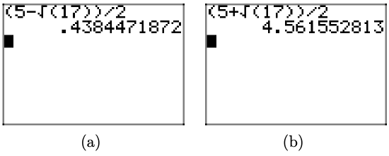
It remains to compare these with the graphical solutions found in part (c). So, enter the solution \((5-\sqrt{( } 17) ) /(2)\) in your calculator screen, as shown in Figure \(\PageIndex{8}\)(a). Enter \((5+\sqrt{( } 17) ) /(2)\), as shown in Figure \(\PageIndex{8}\)(b). Thus,

\[\(\frac{5-\sqrt{17}}{2} \approx 0.4384471872 \quad\) and \(\quad \frac{5+\sqrt{17}}{2} \approx 4.561552813\) \nonumber \]

Note the close agreement with the approximations found in part (c).

Figure \(\PageIndex{8}\). Approximating the exact solutions.

Let’s look at another example.

Example \(\PageIndex{5}\)

Solve the following equation for x, both graphically and analytically \[\frac{1}{x+2}-\frac{x}{2-x}=\frac{x+6}{x^{2}-4} \nonumber \]

Solution

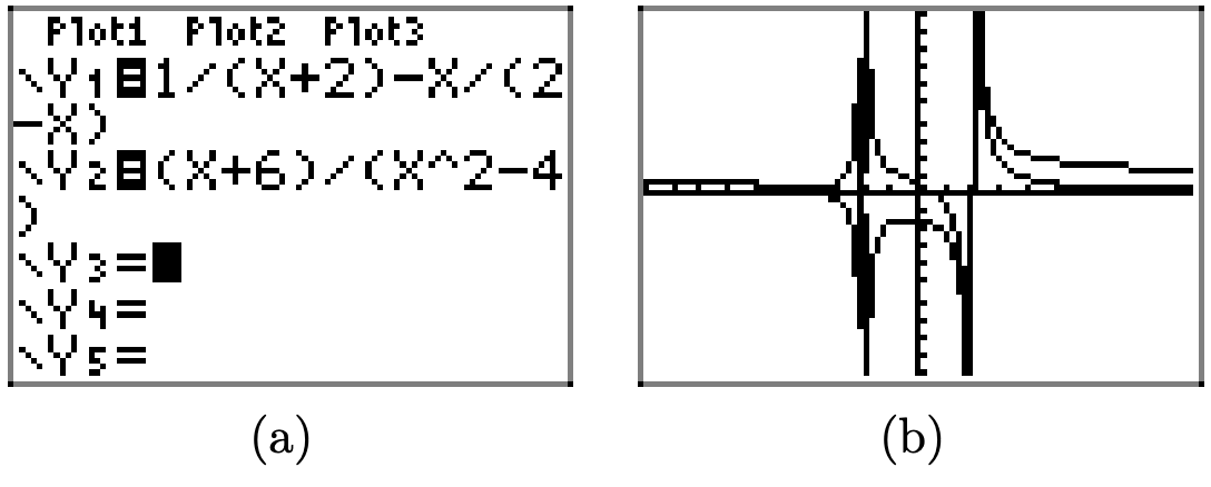
We start the graphical solution in the usual manner, loading the left- and right-hand sides of equation (11) into Y1 and Y2, as shown in Figure \(\PageIndex{9}\)(a). Note that in the resulting plot, shown in Figure \(\PageIndex{9}\)(b), it is very difficult to interpret where the graph of the left-hand side intersects the graph of the right-hand side of equation (11).

Figure \(\PageIndex{9}\). Sketch the left- and right-hand sides of equation (11).

In this situation, a better strategy is to make one side of equation (11) equal to zero.

\[\frac{1}{x+2}-\frac{x}{2-x}-\frac{x+6}{x^{2}-4}=0 \nonumber \]

Our approach will now change. We’ll plot the left-hand side of equation (12), then find where the left-hand side is equal to zero; that is, we’ll find where the graph of the left-hand side of equation (12) intercepts the x-axis.

With this thought in mind, load the left-hand side of equation (12) into Y1, as shown in Figure \(\PageIndex{10}\)(a). Note that the graph in Figure \(\PageIndex{10}\)(b) appears to have only one vertical asymptote at x = −2 (some cancellation must remove the factor of x − 2 from the denominator when you combine the terms of the left-hand side of equation (12)3 ). Further, when you use the zero utility in the CALC menu of the graphing calculator, there appears to be a zero at x = −4, as shown in Figure \(\PageIndex{10}\)(b).

Figure \(\PageIndex{10}\). Finding the zero of the left-hand side of equation (12).

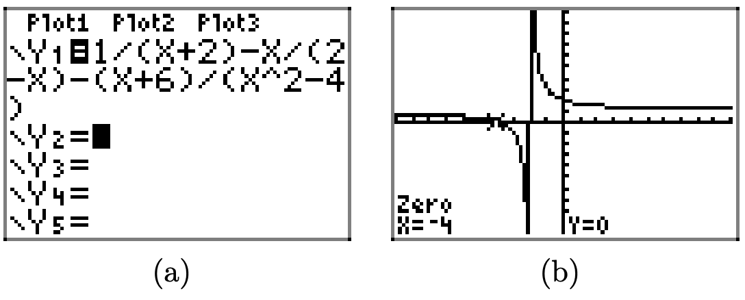
Therefore, equation (12) seems to have only one solution, namely x = 4.

Next, let’s seek an analytical solution of equation (11). We’ll need to factor the denominators in order to discover a common denominator.

\[\frac{1}{x+2}-\frac{x}{2-x}=\frac{x+6}{(x+2)(x-2)} \nonumber \]

It’s tempting to use a denominator of \((x + 2)(2 − x)(x − 2)\). However, the denominator of the second term on the left-hand side of this last equation, 2 − x, is in a different order than the factors in the other denominators, x−2 and x+2, so let’s perform a sign change on this term and reverse the order. We will negate the fraction bar and negate the denominator. That’s two sign changes, so the term remains unchanged when we write

\[\frac{1}{x+2}+\frac{x}{x-2}=\frac{x+6}{(x+2)(x-2)} \nonumber \]

Now we see that a common denominator of (x + 2)(x − 2) will suffice. Let’s multiply both sides of the last equation by \((x + 2)(x − 2)\).

\[\begin{aligned}\color{blue}{(x+2)(x-2)}\left[\frac{1}{x+2}+\frac{x}{x-2}\right] &=\left[\frac{x+6}{(x+2)(x-2)}\right]\color{blue}{(x+2)(x-2)} \\\color{blue}{(x+2)(x-2)}\left[\frac{1}{x+2}\right]+\color{blue}{(x+2)(x-2)}\left[\frac{x}{x-2}\right] &=\left[\frac{x+6}{(x+2)(x-2)}\right]\color{blue}{(x+2)(x-2)} \end{aligned} \nonumber \]

Cancel.

\[\begin{aligned}\color{blue}{(x+2)(x-2)}\left[\frac{1}{x+2}\right]+\color{blue}{(x+2)(x-2)}\left[\frac{x}{x-2}\right] &=\left[\frac{x+6}{(x+2)(x-2)}\right]\color{blue}{(x+2)(x-2)} \\(x-2)+x(x+2) &=x+6 \end{aligned} \nonumber \]

Simplify.

\[\begin{array}{r}{x-2+x^{2}+2 x=x+6} \\ {x^{2}+3 x-2=x+6}\end{array} \nonumber \]

This last equation is nonlinear because of the presence of a power of x larger than 1 (note the \(x^2\) term). Therefore, the strategy is to make one side of the equation equal to zero. We will subtract x and subtract 6 from both sides of the equation.

\[\begin{aligned} x^{2}+3 x-2-x-6 &=0 \\ x^{2}+2 x-8 &=0 \end{aligned} \nonumber \]

The left-hand side is a quadratic trinomial with ac = (1)(−8) = −8. The integer pair 4 and −2 have product −8 and sum 2. Thus,

\[(x+4)(x-2)=0 \nonumber \]

Using the zero product property, either

\[x+4=0 \quad \text { or } \quad x-2=0 \nonumber \]

so \[x=-4 \quad \text { or } \quad x=2 \nonumber \]

The fact that we have found two answers using an analytical method is troubling. After all, the graph in Figure \(\PageIndex{10}\)(b) indicates only one solution, namely x = −4. It is comforting that one of our analytical solutions is also x = −4, but it is still disconcerting that our analytical approach reveals a second “answer,” namely x = 2.

However, notice that we haven’t paid any attention to the restrictions caused by denominators up to this point. Indeed, careful consideration of equation (11) reveals factors of x+2 and x−2 in the denominators. Hence, x = −2 and x = 2 are restrictions.

Note that one of our answers, namely x = 2, is a restricted value. It will make some of the denominators in equation (11) equal to zero, so it cannot be a solution. Thus, the only viable solution is x = −4. One can certainly check this solution by hand, but let’s use the graphing calculator to assist us in the check.

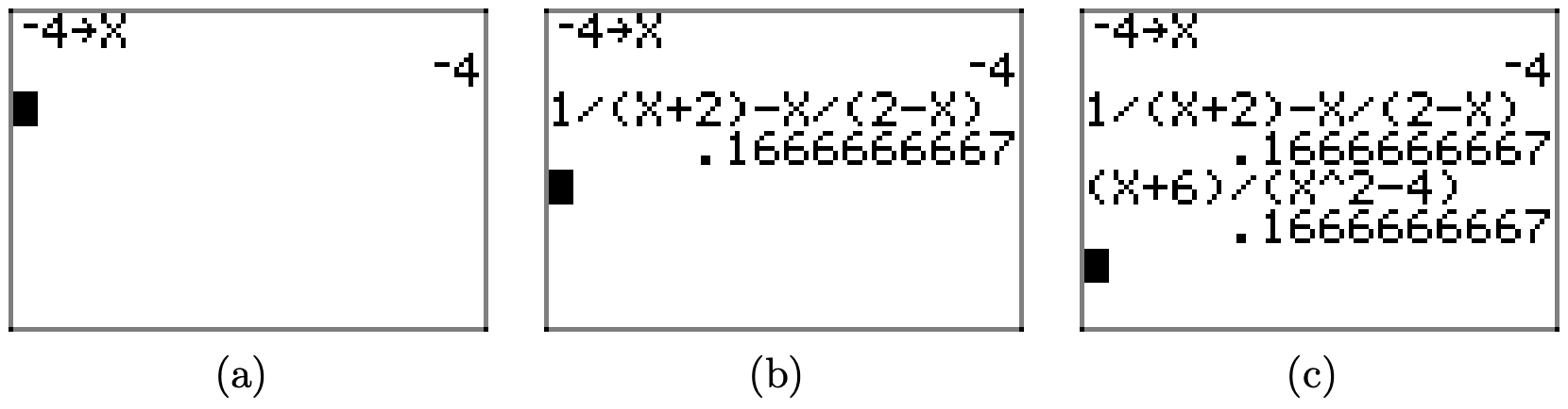
First, enter -4, press the STO\(\blacktriangleright\) button, press X, then press ENTER to execute the resulting command and store -4 in the variable X. The result is shown in Figure \(\PageIndex{11}\)(a).

Next, we calculate the value of the left-hand side of equation (11) at this value of X. Enter the left-hand side of equation (11) as 1/(X+2)-X/(2-X), then press the ENTER key to execute the statement and produce the result shown in Figure \(\PageIndex{11}\)(b).

Finally, enter the right-hand side of equation (11) as (X+6)/(xˆ2-4) and press the ENTER key to execute the statement. The result is shown in Figure \(\PageIndex{11}\)(c). Note that both sides of the equation equal .1666666667 at X=-4. Thus, the solution x = −4 checks.

Figure \(\PageIndex{11}\). Using the graphing calculator to check the solution x = −4 of equation (11).

Exercise

For each of the rational functions given in Exercises 1-6, perform each of the following tasks.

1. Set up a coordinate system on graph paper. Label and scale each axis. Remember to draw all lines with a ruler.
2. Plot the zero of the rational function on your coordinate system and label it with its coordinates. Plot the vertical and horizontal asymptotes on your coordinate system and label them with their equations. Use this information (and your graphing calculator) to draw the graph of f .
3. Plot the horizontal line y = k on your coordinate system and label this line with its equation.
4. Use your calculator’s intersect utility to help determine the solution of f(x) = k. Label this point on your graph with its coordinates.
5. Solve the equation f(x) = k algebraically, placing the work for this solution on your graph paper next to your coordinate system containing the graphical solution. Do the answers agree?

Exercise \(\PageIndex{1}\)

\(f(x) = \frac{x−1}{x+2}\); k = 3

Answer

\(x = −\frac{7}{2}\)

Exercise \(\PageIndex{2}\)

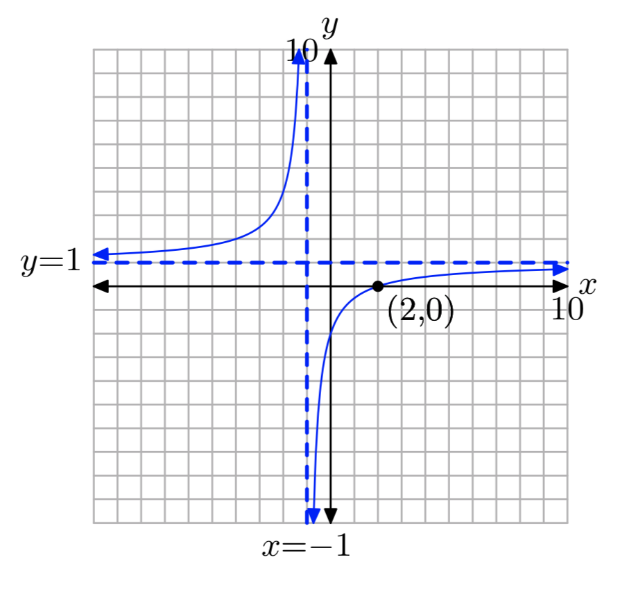
\(f(x) = \frac{x+1}{x−2}\); k = −3

Exercise \(\PageIndex{3}\)

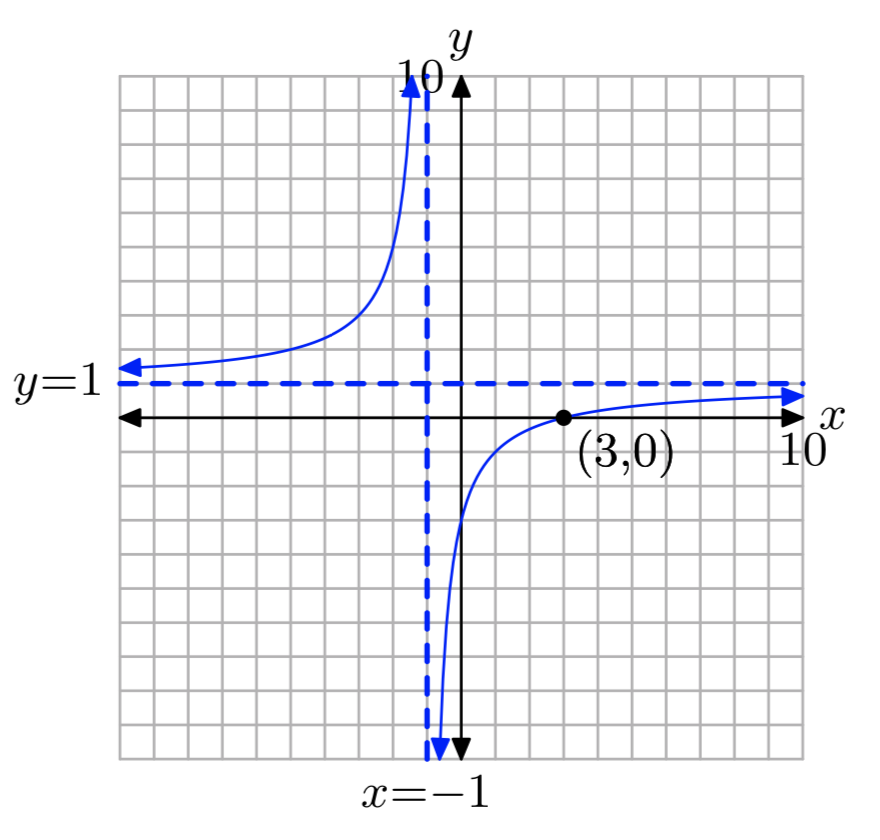
\(f(x) = \frac{x+1}{3−x}\); k = 2

Answer

\(x = \frac{5}{3}\)

Exercise \(\PageIndex{4}\)

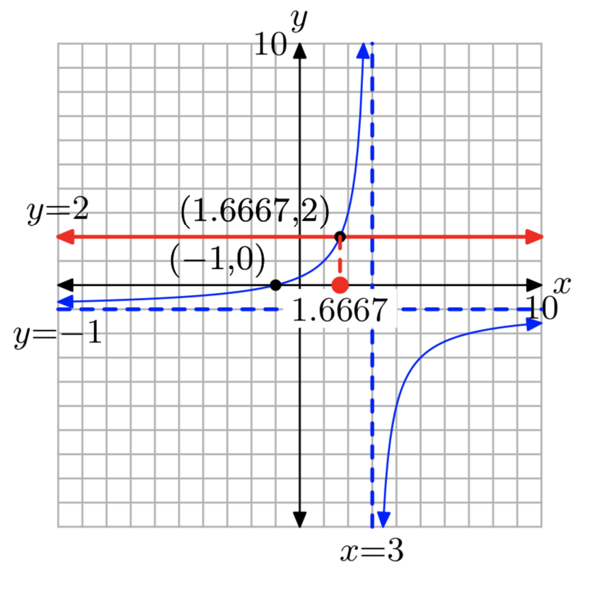
\(f(x) = \frac{x+3}{2−x}\); k = 2

Exercise \(\PageIndex{5}\)

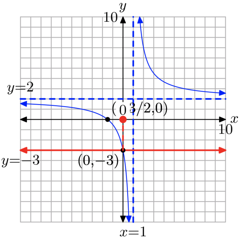
\(f(x) = \frac{2x+3}{x−1}\); k = −3

Answer

x = 0

Exercise \(\PageIndex{6}\)

\(f(x)= \frac{5−2x}{x−1}\); k = 3

In Exercises 7-14, use a strictly algebraic technique to solve the equation f(x) = k for the given function and value of k. You are encouraged to check your result with your calculator.

Exercise \(\PageIndex{7}\)

\(f(x) = \frac{16x−9}{2x−1}\); k = 8

Answer

none

Exercise \(\PageIndex{8}\)

\(f(x) = \frac{10x−3}{7x+7}\); k = 1

Exercise \(\PageIndex{9}\)

\(f(x) = \frac{5x+8}{4x+1}\); k = −11

Answer

\(−\frac{19}{49}\)

Exercise \(\PageIndex{10}\)

\(f(x) = −\frac{6x−11}{7x−2}\); k = −6

Exercise \(\PageIndex{11}\)

\(f(x) = −\frac{35x}{7x+1​​2}\); k = −5

Answer

none

Exercise \(\PageIndex{12}\)

\(f(x) = −\frac{66x−5}{6x−10}\); k = −11

Exercise \(\PageIndex{13}\)

\(f(x) = \frac{8x+2}{x−11}\); k = 11

Answer

41

Exercise \(\PageIndex{14}\)

\(f(x) = \frac{36x−7}{3x−4}\); k = 12

In Exercises 15-20, use a strictly algebraic technique to solve the given equation. You are encouraged to check your result with your calculator.

Exercise \(\PageIndex{15}\)

\(\frac{x}{7}+\frac{8}{9} = −\frac{8}{7}\)

Answer

\(−\frac{128}{9}\)

Exercise \(\PageIndex{16}\)

\(\frac{x}{3}+\frac{9}{2} = −\frac{3}{8}\)

Exercise \(\PageIndex{17}\)

\(−\frac{57}{x}=27−\frac{40}{x^2}\)

Answer

\(−\frac{8}{5}, \frac{3}{9}\)

Exercise \(\PageIndex{18}\)

\(−\frac{117}{x} = 54+\frac{54}{x^2}\)

Exercise \(\PageIndex{19}\)

\(\frac{7}{x} = 4−\frac{3}{x^2}\)

Answer

\(\frac{7+\sqrt{97}}{8}, \frac{7−\sqrt{97}}{8}\)

Exercise \(\PageIndex{20}\)

\(\frac{3}{x^2} = 5−\frac{3}{x}\)

For each of the rational functions given in Exercises 21-26, perform each of the following tasks.

1. Set up a coordinate system on graph paper. Label and scale each axis. Re- member to draw all lines with a ruler.
2. Plot the zero of the rational function on your coordinate system and label it with its coordinates. You may use your calculator’s zero utility to find this, if you wish.
3. Plot the vertical and horizontal asymptotes on your coordinate system and label them with their equations. Use the asymptote and zero information (and your graphing calculator) to draw the graph of f.
4. Plot the horizontal line y = k on your coordinate system and label this line with its equation.
5. Use your calculator’s intersect utility to help determine the solution of f(x) = k. Label this point on your graph with its coordinates.
6. Solve the equation f(x) = k algebraically, placing the work for this solution on your graph paper next to your coordinate system containing the graphical solution. Do the answers agree?

Exercise \(\PageIndex{21}\)

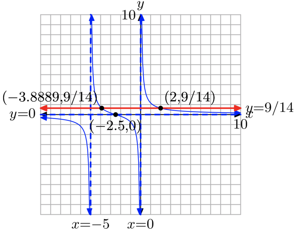
\(f(x) = \frac{1}{x}+\frac{1}{x+5}\), \(k = \frac{9}{14}\)

Answer

\(x = −\frac{35}{9}\) or x = 2

Exercise \(\PageIndex{22}\)

\(f(x) = \frac{1}{x}+\frac{1}{x−2}\), \(k = \frac{8}{15}\)

Exercise \(\PageIndex{23}\)

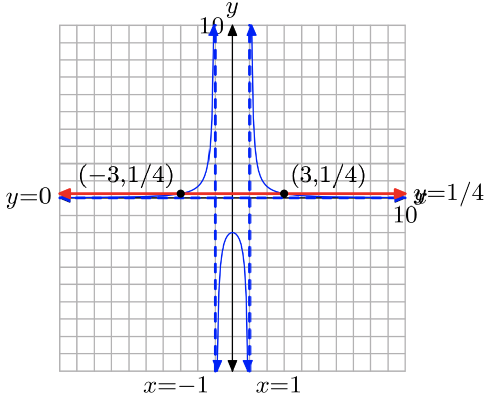
\(f(x) = \frac{1}{x−1}−\frac{1}{x+1}\), \(k = \frac{1}{4}\)

Answer

x = −3 or x = 3

Exercise \(\PageIndex{24}\)

\(f(x) = \frac{1}{x−1}−\frac{1}{x+2}\), \(k = \frac{1}{6}\)

Exercise \(\PageIndex{25}\)

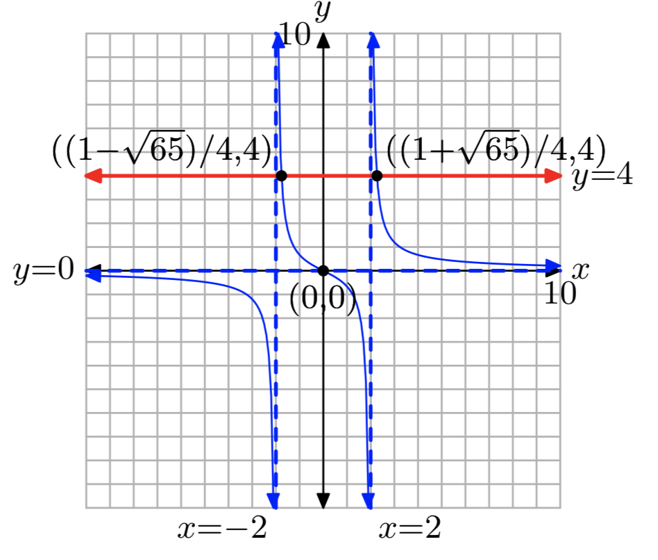
\(f(x) = \frac{1}{x−2}+\frac{1}{x+2}\), k = 4

Answer

\(x = \frac{1+\sqrt{65}}{4}, \frac{1−\sqrt{65}}{4}\)

Exercise \(\PageIndex{26}\)

\(f(x) = \frac{1}{x−3}+\frac{1}{x+2}\), k = 5

In Exercises 27-34, use a strictly algebraic technique to solve the given equation. You are encouraged to check your result with your calculator.

Exercise \(\PageIndex{27}\)

\(\frac{2}{x+1}+\frac{4}{x+2} = −3\)

Answer

\(\frac{−15+\sqrt{57}}{6}, \frac{−15−\sqrt{57}}{6}\)

Exercise \(\PageIndex{28}\)

\(\frac{2}{x−5}−\frac{7}{x−7} = 9\)

Exercise \(\PageIndex{29}\)

\(\frac{3}{x+9}−\frac{2}{x+7} = −3\)

Answer

\(\frac{−49+\sqrt{97}}{6}, \frac{−49−\sqrt{97}}{6}\)

Exercise \(\PageIndex{30}\)

\(\frac{3}{x+9}−\frac{6}{x+7} = 9\)

Exercise \(\PageIndex{31}\)

\(\frac{2}{x+9}+\frac{2}{x+6} = −1\)

Answer

−7, −12

Exercise \(\PageIndex{32}\)

\(\frac{5}{x−6}−\frac{8}{x−7} = −1\)

Exercise \(\PageIndex{33}\)

\(\frac{3}{x+3}+\frac{6}{x+2} = −2\)

Answer

\(\frac{−19+\sqrt{73}}{4}, \frac{−19−\sqrt{73}}{4}\)

Exercise \(\PageIndex{34}\)

\(\frac{2}{x−4}−\frac{2}{x−1} = 1\)

For each of the equations in Exercises 35-40, perform each of the following tasks.

1. Follow the lead of Example 10 in the text. Make one side of the equation equal to zero. Load the nonzero side into your calculator and draw its graph.
2. Determine the vertical asymptotes of by analyzing the equation and the resulting graph on your calculator. Use the TABLE feature of your calculator to determine any horizontal asymptote behavior.
3. Use the zero finding utility in the CALC menu to determine the zero of the nonzero side of the resulting equation.
4. Set up a coordinate system on graph paper. Label and scale each axis. Remember to draw all lines with a ruler.Draw the graph of the nonzero side of the equation. Draw the vertical and horizontal asymptotes and label them with their equations. Plot the x-intercept and label it with its coordinates.
5. Use an algebraic technique to deter- mine the solution of the equation and compare it with the solution found by the graphical analysis above.

Exercise \(\PageIndex{35}\)

\(\frac{x}{x+1}+\frac{8}{x^2−2x−3} = \frac{2}{x−3}\)

Answer

x = 2

Exercise \(\PageIndex{36}\)

\(\frac{x}{x+4}−\frac{2}{x+1} = \frac{12}{x^2+5x+4}\)

Exercise \(\PageIndex{37}\)

\(\frac{x}{x+1}−\frac{4}{2x+1} = \frac{2x−1}{2x^2+3x+2}\)

Answer

x = 3

Exercise \(\PageIndex{38}\)

\(\frac{2x}{x−4}−\frac{1}{x+1} = \frac{4x+24}{x^2−3x−4}\)

Exercise \(\PageIndex{39}\)

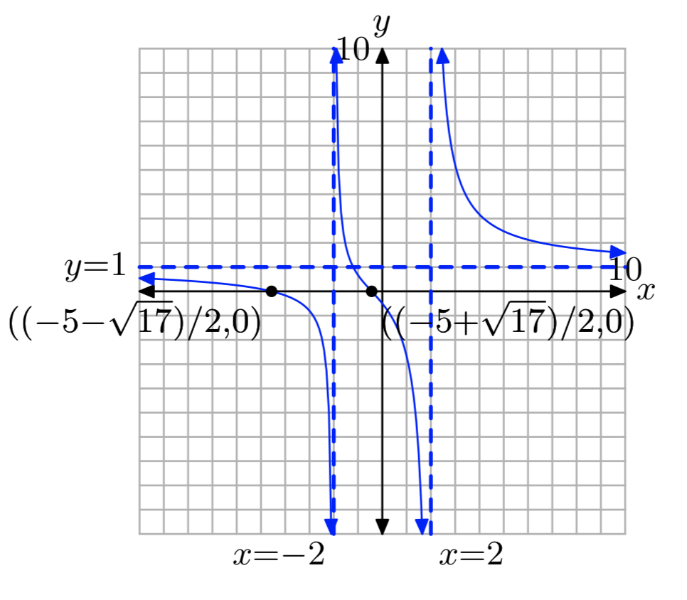
\(\frac{x}{x−2}+\frac{3}{x+2} = \frac{8}{4−x^2}\)

Answer

\(x = \frac{5−\sqrt{17}}{2}, \frac{−5−\sqrt{17}}{2}\)

Exercise \(\PageIndex{40}\)

\(\frac{x}{x−6​​​​​1​}−\frac{4}{x+1} = \frac{x−6}{1−x^2}\)

In Exercises 41-68, use a strictly algebraic technique to solve the given equation. You are encouraged to check your result with your calculator.

Exercise \(\PageIndex{41}\)

\(\frac{x}{3x−9}−\frac{9}{x} = \frac{1}{x−3}\)

Answer

27

Exercise \(\PageIndex{42}\)

\(\frac{5x}{x+2}+\frac{5}{x−5} = \frac{x+6}{x^2−3x−10}\)

Exercise \(\PageIndex{43}\)

\(\frac{3x}{x+2}−\frac{7}{x} = −\frac{1}{2x+4}\)

Answer

\(\frac{7}{2}, −\frac{4}{3}\)

Exercise \(\PageIndex{44}\)

\(\frac{4x}{x+6}−\frac{4}{x+4} = \frac{x−4}{x^2+10x+24}\)

Exercise \(\PageIndex{45}\)

\(\frac{x}{x−5}+\frac{9}{4−x} = \frac{x+5}{x^2−9x+20}\)

Answer

10

Exercise \(\PageIndex{46}\)

\(\frac{6x}{x−5}−\frac{2}{x−3} = \frac{x−8}{x^2−8x+15}\)

Exercise \(\PageIndex{47}\)

\(\frac{2x}{x−4}+\frac{5}{2−x} = \frac{x+8}{x^2−6x+8}\)

Answer

3

Exercise \(\PageIndex{48}\)

\(\frac{x}{x−7}−\frac{8}{5−x} = \frac{x+7}{x^2−12x+35}\)

Exercise \(\PageIndex{49}\)

\(−\frac{x}{2x+2}−\frac{6}{x} = −\frac{2}{x+1}\)

Answer

−6, −2

Exercise \(\PageIndex{50}\)

\(\frac{7x}{x+3}−\frac{4}{2−x} = \frac{x+8}{x^2+x−6}\)​​​​​​

Exercise \(\PageIndex{51}\)

\(\frac{2x}{x+5}−\frac{2}{6−x} = \frac{x−2}{x^2−x−30}\)

Answer

4, \(\frac{3}{2}\)

Exercise \(\PageIndex{52}\)

\(\frac{4x}{x+1}+\frac{6}{x+3} = \frac{x−9}{x^2+4x+3}\)

Exercise \(\PageIndex{53}\)

\(\frac{x}{x+7}−\frac{2}{x+5}​​​​​​​ = \frac{x+1}{x^2+12x+35}\)

Answer

3

Exercise \(\PageIndex{54}\)

\(\frac{5x}{6x+4}+\frac{6}{x} = \frac{1}{3x+2}\)

Exercise \(\PageIndex{55}\)

\(\frac{2x}{3x+9​​​​​​​}−\frac{4}{x} = −\frac{2}{x+3}\)

Answer

6

Exercise \(\PageIndex{56}\)

\(\frac{7x}{x+1}−\frac{4}{x+2} = \frac{x+6}{x^2+3x+2}\)

Exercise \(\PageIndex{57}\)

\(\frac{x}{2x−8​​​​​​​} + \frac{8}{x} = \frac{2}{x−4}\)

Answer

−16

Exercise \(\PageIndex{58}\)

\(\frac{3x}{x−6}+\frac{6}{x−6} = \frac{x+2}{x^2−12x+36}\)

Exercise \(\PageIndex{59}\)

\(\frac{x}{x+2}+\frac{2}{x} = −\frac{5}{2x+4}\)

Answer

\(\frac{−9+\sqrt{17}}{4}, \frac{−9−\sqrt{17}}{4}\)

Exercise \(\PageIndex{60}\)

\(\frac{4x}{x−2}+\frac{2}{2−x} = \frac{x+4}{x^2−4x+4}\)

Exercise \(\PageIndex{61}\)

\(−\frac{2x}{3x−9​​​​​​​}−\frac{3}{x} = −\frac{2}{x−3}\)

Answer

\(−\frac{9}{2}\)

Exercise \(\PageIndex{62}\)

\(\frac{2x}{x+1}−\frac{2}{x} = \frac{1}{2x+2}\)

Exercise \(\PageIndex{63}\)

\(\frac{x}{x+1}+\frac{5}{x} = \frac{1}{4x+4}\)

Answer

\(\frac{−19+\sqrt{41}}{8}, \frac{−19−\sqrt{41}}{8}\)

Exercise \(\PageIndex{64}\)

\(\frac{2x}{x−4}−\frac{8}{x−7} = \frac{x+2}{x^2−11x+28}\)

Exercise \(\PageIndex{65}\)

\(−\frac{9x}{x−2}+\frac{2}{x} = −\frac{2}{4x−1}\)

Answer

\(\frac{9}{2}\), 5

Exercise \(\PageIndex{66}\)

\(\frac{2x}{x−3​​​​​​​}−\frac{4}{4−x} = \frac{x−9}{x^2−7x+12}\)​​​​​​​

Exercise \(\PageIndex{67}\)

\(\frac{4x}{x+6}−\frac{5}{7−x} = \frac{x−5}{x^2−x−42}\)

Answer

\(\frac{7}{2}, \frac{5}{2}\)

Exercise \(\PageIndex{68}\)

\(\frac{x}{x−1​​​​​​​}−\frac{4}{x} = \frac{1}{5x−5}\)

​​​​​​​