11.6: Solving Systems of Nonlinear Equations
- Page ID
- 5192
\( \newcommand{\vecs}[1]{\overset { \scriptstyle \rightharpoonup} {\mathbf{#1}} } \)
\( \newcommand{\vecd}[1]{\overset{-\!-\!\rightharpoonup}{\vphantom{a}\smash {#1}}} \)
\( \newcommand{\dsum}{\displaystyle\sum\limits} \)
\( \newcommand{\dint}{\displaystyle\int\limits} \)
\( \newcommand{\dlim}{\displaystyle\lim\limits} \)
\( \newcommand{\id}{\mathrm{id}}\) \( \newcommand{\Span}{\mathrm{span}}\)
( \newcommand{\kernel}{\mathrm{null}\,}\) \( \newcommand{\range}{\mathrm{range}\,}\)
\( \newcommand{\RealPart}{\mathrm{Re}}\) \( \newcommand{\ImaginaryPart}{\mathrm{Im}}\)
\( \newcommand{\Argument}{\mathrm{Arg}}\) \( \newcommand{\norm}[1]{\| #1 \|}\)
\( \newcommand{\inner}[2]{\langle #1, #2 \rangle}\)
\( \newcommand{\Span}{\mathrm{span}}\)
\( \newcommand{\id}{\mathrm{id}}\)
\( \newcommand{\Span}{\mathrm{span}}\)
\( \newcommand{\kernel}{\mathrm{null}\,}\)
\( \newcommand{\range}{\mathrm{range}\,}\)
\( \newcommand{\RealPart}{\mathrm{Re}}\)
\( \newcommand{\ImaginaryPart}{\mathrm{Im}}\)
\( \newcommand{\Argument}{\mathrm{Arg}}\)
\( \newcommand{\norm}[1]{\| #1 \|}\)
\( \newcommand{\inner}[2]{\langle #1, #2 \rangle}\)
\( \newcommand{\Span}{\mathrm{span}}\) \( \newcommand{\AA}{\unicode[.8,0]{x212B}}\)
\( \newcommand{\vectorA}[1]{\vec{#1}} % arrow\)
\( \newcommand{\vectorAt}[1]{\vec{\text{#1}}} % arrow\)
\( \newcommand{\vectorB}[1]{\overset { \scriptstyle \rightharpoonup} {\mathbf{#1}} } \)
\( \newcommand{\vectorC}[1]{\textbf{#1}} \)
\( \newcommand{\vectorD}[1]{\overrightarrow{#1}} \)
\( \newcommand{\vectorDt}[1]{\overrightarrow{\text{#1}}} \)
\( \newcommand{\vectE}[1]{\overset{-\!-\!\rightharpoonup}{\vphantom{a}\smash{\mathbf {#1}}}} \)
\( \newcommand{\vecs}[1]{\overset { \scriptstyle \rightharpoonup} {\mathbf{#1}} } \)
\(\newcommand{\longvect}{\overrightarrow}\)
\( \newcommand{\vecd}[1]{\overset{-\!-\!\rightharpoonup}{\vphantom{a}\smash {#1}}} \)
\(\newcommand{\avec}{\mathbf a}\) \(\newcommand{\bvec}{\mathbf b}\) \(\newcommand{\cvec}{\mathbf c}\) \(\newcommand{\dvec}{\mathbf d}\) \(\newcommand{\dtil}{\widetilde{\mathbf d}}\) \(\newcommand{\evec}{\mathbf e}\) \(\newcommand{\fvec}{\mathbf f}\) \(\newcommand{\nvec}{\mathbf n}\) \(\newcommand{\pvec}{\mathbf p}\) \(\newcommand{\qvec}{\mathbf q}\) \(\newcommand{\svec}{\mathbf s}\) \(\newcommand{\tvec}{\mathbf t}\) \(\newcommand{\uvec}{\mathbf u}\) \(\newcommand{\vvec}{\mathbf v}\) \(\newcommand{\wvec}{\mathbf w}\) \(\newcommand{\xvec}{\mathbf x}\) \(\newcommand{\yvec}{\mathbf y}\) \(\newcommand{\zvec}{\mathbf z}\) \(\newcommand{\rvec}{\mathbf r}\) \(\newcommand{\mvec}{\mathbf m}\) \(\newcommand{\zerovec}{\mathbf 0}\) \(\newcommand{\onevec}{\mathbf 1}\) \(\newcommand{\real}{\mathbb R}\) \(\newcommand{\twovec}[2]{\left[\begin{array}{r}#1 \\ #2 \end{array}\right]}\) \(\newcommand{\ctwovec}[2]{\left[\begin{array}{c}#1 \\ #2 \end{array}\right]}\) \(\newcommand{\threevec}[3]{\left[\begin{array}{r}#1 \\ #2 \\ #3 \end{array}\right]}\) \(\newcommand{\cthreevec}[3]{\left[\begin{array}{c}#1 \\ #2 \\ #3 \end{array}\right]}\) \(\newcommand{\fourvec}[4]{\left[\begin{array}{r}#1 \\ #2 \\ #3 \\ #4 \end{array}\right]}\) \(\newcommand{\cfourvec}[4]{\left[\begin{array}{c}#1 \\ #2 \\ #3 \\ #4 \end{array}\right]}\) \(\newcommand{\fivevec}[5]{\left[\begin{array}{r}#1 \\ #2 \\ #3 \\ #4 \\ #5 \\ \end{array}\right]}\) \(\newcommand{\cfivevec}[5]{\left[\begin{array}{c}#1 \\ #2 \\ #3 \\ #4 \\ #5 \\ \end{array}\right]}\) \(\newcommand{\mattwo}[4]{\left[\begin{array}{rr}#1 \amp #2 \\ #3 \amp #4 \\ \end{array}\right]}\) \(\newcommand{\laspan}[1]{\text{Span}\{#1\}}\) \(\newcommand{\bcal}{\cal B}\) \(\newcommand{\ccal}{\cal C}\) \(\newcommand{\scal}{\cal S}\) \(\newcommand{\wcal}{\cal W}\) \(\newcommand{\ecal}{\cal E}\) \(\newcommand{\coords}[2]{\left\{#1\right\}_{#2}}\) \(\newcommand{\gray}[1]{\color{gray}{#1}}\) \(\newcommand{\lgray}[1]{\color{lightgray}{#1}}\) \(\newcommand{\rank}{\operatorname{rank}}\) \(\newcommand{\row}{\text{Row}}\) \(\newcommand{\col}{\text{Col}}\) \(\renewcommand{\row}{\text{Row}}\) \(\newcommand{\nul}{\text{Nul}}\) \(\newcommand{\var}{\text{Var}}\) \(\newcommand{\corr}{\text{corr}}\) \(\newcommand{\len}[1]{\left|#1\right|}\) \(\newcommand{\bbar}{\overline{\bvec}}\) \(\newcommand{\bhat}{\widehat{\bvec}}\) \(\newcommand{\bperp}{\bvec^\perp}\) \(\newcommand{\xhat}{\widehat{\xvec}}\) \(\newcommand{\vhat}{\widehat{\vvec}}\) \(\newcommand{\uhat}{\widehat{\uvec}}\) \(\newcommand{\what}{\widehat{\wvec}}\) \(\newcommand{\Sighat}{\widehat{\Sigma}}\) \(\newcommand{\lt}{<}\) \(\newcommand{\gt}{>}\) \(\newcommand{\amp}{&}\) \(\definecolor{fillinmathshade}{gray}{0.9}\)By the end of this section, you will be able to:
- Solve a system of nonlinear equations using graphing
- Solve a system of nonlinear equations using substitution
- Solve a system of nonlinear equations using elimination
- Use a system of nonlinear equations to solve applications
Before you get started, take this readiness quiz.
- Solve the system by graphing: \(\left\{\begin{array}{l}{x-3 y=-3} \\ {x+y=5}\end{array}\right.\).
If you missed this problem, review Example 4.2. - Solve the system by substitution: \(\left\{\begin{array}{l}{x-4 y=-4} \\ {-3 x+4 y=0}\end{array}\right.\)
If you missed this problem, review Example 4.7. - Solve the system by elimination: \(\left\{\begin{array}{l}{3 x-4 y=-9} \\ {5 x+3 y=14}\end{array}\right.\)
If you missed this problem, review Example 4.9.
Solve a System of Nonlinear Equations using Graphing
We learned how to solve systems of linear equations with two variables by graphing, substitution and elimination. We will be using these same methods as we look at nonlinear systems of equations with two equations and two variables. A system of nonlinear equations is a system where at least one of the equations is not linear.
For example each of the following systems is a system of nonlinear equations.
\(\left\{\begin{array}{l}{x^{2}+y^{2}=9} \\ {x^{2}-y=9}\end{array}\right. \left\{\begin{array}{l}{9 x^{2}+y^{2}=9} \\ {y=3 x-3}\end{array}\right. \left\{\begin{array}{l}{x+y=4} \\ {y=x^{2}+2}\end{array}\right.\)
A system of nonlinear equations is a system where at least one of the equations is not linear.
Just as with systems of linear equations, a solution of a nonlinear system is an ordered pair that makes both equations true. In a nonlinear system, there may be more than one solution. We will see this as we solve a system of nonlinear equations by graphing.
When we solved systems of linear equations, the solution of the system was the point of intersection of the two lines. With systems of nonlinear equations, the graphs may be circles, parabolas or hyperbolas and there may be several points of intersection, and so several solutions. Once you identify the graphs, visualize the different ways the graphs could intersect and so how many solutions there might be.
To solve systems of nonlinear equations by graphing, we use basically the same steps as with systems of linear equations modified slightly for nonlinear equations. The steps are listed below for reference.
Solve a System of Nonlinear Equations by Graphing.
- Identify the graph of each equation. Sketch the possible options for intersection.
- Graph the first equation.
- Graph the second equation on the same rectangular coordinate system.
- Determine whether the graphs intersect.
- Identify the points of intersection.
- Check that each ordered pair is a solution to both original equations.
Solve the system by graphing: \(\left\{\begin{array}{l}{x-y=-2} \\ {y=x^{2}}\end{array}\right.\)
Solution:
| Identify each graph. | \(\left\{\begin{array}{ll}{x-y=-2} & {\text { line }} \\ {y=x^{2}} & {\text { parabola }}\end{array}\right.\) |
| Sketch the possible options for intersection of a parabola and a line. | 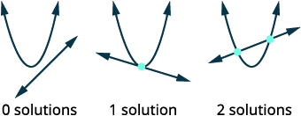 |
|
Graph the line, \(x-y=-2\). Slope-intercept form \(y=x+2\). Graph the parabola, \(y=x^{2}\). |
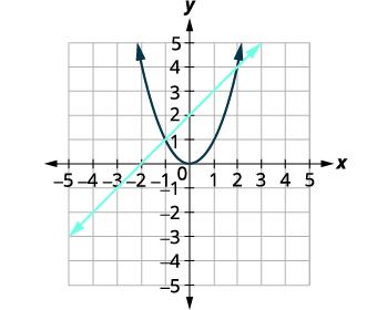 |
| Identify the points of intersection. | The points of intersection appear to be \((2,3)\) and \((-1,1)\). |
|
Check to make sure each solution makes both equations true. \((2,4)\) \(\begin{array} {r l } {x-y=-2}\quad\quad {y=x^{2}} \\ {2-4\stackrel{?}{=}-2}\quad\quad {4\stackrel{?}{=}2^{2}} \\ {-2 = -2}\quad\quad\:{4 = 4} \end{array}\) \((-1,1)\) \(\begin{array} {l l } {x-y=-2}\quad\quad {y=x^{2}} \\ {-1-1\stackrel{?}{=}-2}\:\quad {1\stackrel{?}{=}(-1)^{2}} \\ {-2 = -2}\quad\quad\quad{1 = 1} \end{array}\) |
|
| The solutions are \((2,4)\) and \((-1,1)\). |
Solve the system by graphing: \(\left\{\begin{array}{l}{x+y=4} \\ {y=x^{2}+2}\end{array}\right.\).
- Answer
-
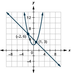
Figure 11.5.3
Solve the system by graphing: \(\left\{\begin{array}{l}{x-y=-1} \\ {y=-x^{2}+3}\end{array}\right.\)
- Answer
-
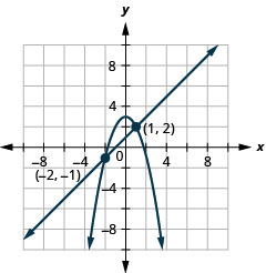
Figure 11.5.4
To identify the graph of each equation, keep in mind the characteristics of the \(x^{2}\) and \(y^{2}\) terms of each conic.
Solve the system by graphing: \(\left\{\begin{array}{l}{y=-1} \\ {(x-2)^{2}+(y+3)^{2}=4}\end{array}\right.\).
Solution:
| Identify each graph. | \(\left\{\begin{array}{ll}{y=-1} & {\text { line }} \\ {(x-2)^{2}+(y+3)^{2}=4} & {\text { circle }}\end{array}\right.\) |
| Sketch the possible options for the intersection of a circle and a line. |  |
|
Graph the circle, \((x-2)^{2}+(y+3)^{2}=4\) Center: \((2,-3)\) radius: \(2\) Graph the line, \(y=-1\). It is a horizontal line. |
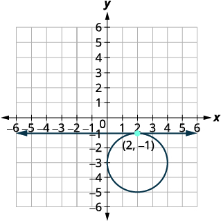 |
| Identify the points of intersection. | The point of intersection appears to be\((2,-1)\). |
|
Check to make sure the solution makes both equations true. \((2,-1)\) \(\begin{array} {r r} {(x-2)^{2}+(y+3)^{2}=4} \quad\quad {y=-1} \\ {(2-2)^{2}+(-1+3)^{2}\stackrel{?}{=}4}\quad{-1=-1} \\ {(0)^{2}+(2)^{2}\stackrel{?}{=}4}\quad\quad\quad\quad\quad \\ {4=4}\quad\quad\quad\quad\quad \end{array}\) |
|
| The solution is \((2,-1)\) |
Solve the system by graphing: \(\left\{\begin{array}{l}{x=-6} \\ {(x+3)^{2}+(y-1)^{2}=9}\end{array}\right.\)
- Answer
-
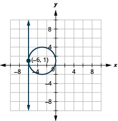
Figure 11.5.7
Solve the system by graphing: \(\left\{\begin{array}{l}{y=4} \\ {(x-2)^{2}+(y+3)^{2}=4}\end{array}\right.\)
- Answer
-
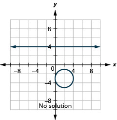
Figure 11.5.8
Solve a System of Nonlinear Equations Using Substitution
The graphing method works well when the points of intersection are integers and so easy to read off the graph. But more often it is difficult to read the coordinates of the points of intersection. The substitution method is an algebraic method that will work well in many situations. It works especially well when it is easy to solve one of the equations for one of the variables.
The substitution method is very similar to the substitution method that we used for systems of linear equations. The steps are listed below for reference.
Solve a System of Nonlinear Equations by Substitution
- Identify the graph of each equation. Sketch the possible options for intersection.
- Solve one of the equations for either variable.
- Substitute the expression from Step 2 into the other equation.
- Solve the resulting equation.
- Substitute each solution in Step 4 into one of the original equations to find the other variable.
- Write each solution as an ordered pair.
- Check that each ordered pair is a solution to both original equations.
Solve the system by using substitution: \(\left\{\begin{array}{l}{9 x^{2}+y^{2}=9} \\ {y=3 x-3}\end{array}\right.\)
Solution:
| Identify each graph. | \(\left\{\begin{array}{ll}{9 x^{2}+y^{2}=9} & {\text { ellipse }} \\ {y=3 x-3} & {\text { line }}\end{array}\right.\) |
| Sketch the possible options for intersection of an ellipse and a line. |  |
| The equation \(y=3x-3\) is solved for \(y\). |  |
 |
|
| Substitute \(3x-3\) for \(y\) in the first equation. |  |
| Solve the equation for \(x\). |  |
 |
|
| Substitute \(x=0\) and \(x=1\) into \(y=3x-3\) to find \(y\)-. |  |
 |
|
| The ordered pairs are \((0,-3), (1,0)\). | |
|
Check both ordered pairs in both equations. \((0,-3)\) \(\begin{array} {r l}{9 x^{2}+y^{2}=9} &\quad { y=3 x-3} \\ {9\cdot0^{2}+(-3)^{2}\stackrel{?}{=}9}&\quad{-3\stackrel{?}{=}3\cdot0-3} \\ {0+9\stackrel{?}{=}9}&\quad{-3\stackrel{?}{=}0-3} \\ {9=9}&\quad{-3=-3} \end{array}\) \((1,0)\) \(\begin{array} {r l}{9 x^{2}+y^{2}=9} &\quad { y=3 x-3} \\ {9\cdot 1^{2}+(0)^{2}\stackrel{?}{=}9}&\quad{0\stackrel{?}{=}3\cdot 1-3} \\ {9+0\stackrel{?}{=}9}&\quad{0\stackrel{?}{=}3-3} \\ {9=9}&\quad{0=0} \end{array}\) |
|
| The solutions are \((0,-3), (1,0)\). |
Solve the system by using substitution: \(\left\{\begin{array}{l}{x^{2}+9 y^{2}=9} \\ {y=\frac{1}{3} x-3}\end{array}\right.\)
- Answer
-
No solution
Solve the system by using substitution: \(\left\{\begin{array}{l}{4 x^{2}+y^{2}=4} \\ {y=x+2}\end{array}\right.\)
- Answer
-
\(\left(-\frac{4}{5}, \frac{6}{5}\right),(0,2)\)
So far, each system of nonlinear equations has had at least one solution. The next example will show another option.
Solve the system by using substitution: \(\left\{\begin{array}{l}{x^{2}-y=0} \\ {y=x-2}\end{array}\right.\)
Solution:
| Identify each graph. | \(\left\{\begin{array}{ll}{x^{2}-y=0} & {\text { parabola }} \\ {y=x-2} & {\text { line }}\end{array}\right.\) |
| Sketch the possible options for intersection of a parabola and a line. | 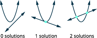 |
| The equation \(y=x-2\) is solved for \(y\). |  |
 |
|
| Substitute \(x-2\) for \(y\) in the first equation. |  |
| Solve the equation for \(x\). |  |
| This doesn't factor easily, so we can check the discriminant. | |
| \(\begin{array}{c}{b^{2}-4 a c} \\ {(-1)^{2}-4 \cdot 1 \cdot 2} \\ {-7}\end{array}\) |
The discriminant is negative, so there is no real solution. The system has no solution. |
Solve the system by using substitution: \(\left\{\begin{array}{l}{x^{2}-y=0} \\ {y=2 x-3}\end{array}\right.\)
- Answer
-
No solution
Solve the system by using substitution: \(\left\{\begin{array}{l}{y^{2}-x=0} \\ {y=3 x-2}\end{array}\right.\)
- Answer
-
\(\left(\frac{4}{9},-\frac{2}{3}\right),(1,1)\)
Solve a System of Nonlinear Equations Using Elimination
When we studied systems of linear equations, we used the method of elimination to solve the system. We can also use elimination to solve systems of nonlinear equations. It works well when the equations have both variables squared. When using elimination, we try to make the coefficients of one variable to be opposites, so when we add the equations together, that variable is eliminated.
The elimination method is very similar to the elimination method that we used for systems of linear equations. The steps are listed for reference.
Solve a System of Equations by Elimination
- Identify the graph of each equation. Sketch the possible options for intersection.
- Write both equations in standard form.
- Make the coefficients of one variable opposites.
Decide which variable you will eliminate.
Multiply one or both equations so that the coefficients of that variable are opposites. - Add the equations resulting from Step 3 to eliminate one variable.
- Solve for the remaining variable.
- Substitute each solution from Step 5 into one of the original equations. Then solve for the other variable.
- Write each solution as an ordered pair.
- Check that each ordered pair is a solution to both original equations.
Solve the system by elimination: \(\left\{\begin{array}{l}{x^{2}+y^{2}=4} \\ {x^{2}-y=4}\end{array}\right.\)
Solution:
| Identify each graph. |  |
| Sketch the possible options for intersection of a circle and a parabola. | 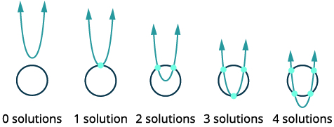 |
| Both equations are in standard form. |  |
| To get opposite coefficients of \(x^{2}\), we will multiply the second equation by \(-1\). |  |
| Simplify. |  |
| Add the two equation to eliminate \(x^{2}\)/ |  |
| Solve for \(y\). |  |
 |
|
| Substitute \(y=0\) and \(y=-1\) into one of the original equations. Then solve for \(x\). |  |
 |
|
| Write each solution as an ordered pair. | The ordered pairs are \((-2,0)(2,0)\). \((\sqrt{3},-1)(-\sqrt{3},-1)\) |
| Check that each ordered pair is a solution to both original equations. | |
| We will leave the checks for each of the four solutions to you. | The solutions are \((-2,0),(2,0),(\sqrt{3},-1)\), and \((-\sqrt{3},-1)\). |
Solve the system by elimination: \(\left\{\begin{array}{l}{x^{2}+y^{2}=9} \\ {x^{2}-y=9}\end{array}\right.\)
- Answer
-
\((-3,0),(3,0),(-2 \sqrt{2},-1),(2 \sqrt{2},-1)\)
Solve the system by elimination: \(\left\{\begin{array}{l}{x^{2}+y^{2}=1} \\ {-x+y^{2}=1}\end{array}\right.\)
- Answer
-
\((-1,0),(0,1),(0,-1)\)
There are also four options when we consider a circle and a hyperbola.
Solve the system by elimination: \(\left\{\begin{array}{l}{x^{2}+y^{2}=7} \\ {x^{2}-y^{2}=1}\end{array}\right.\)
Solution:
| Identify each graph. | \(\left\{\begin{array}{ll}{x^{2}+y^{2}=7} & {\text { circle }} \\ {x^{2}-y^{2}=1} & {\text { hyperbola }}\end{array}\right.\) |
| Sketch the possible options for intersection of a circle and hyperbola. | 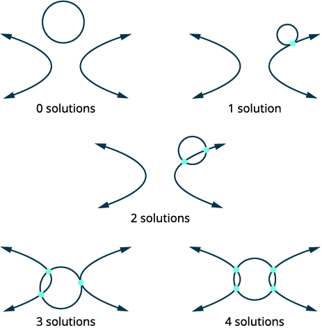 |
| Both equations are in standard form. | \(\left\{\begin{array}{l}{x^{2}+y^{2}=7} \\ {x^{2}-y^{2}=1}\end{array}\right.\) |
| The coefficients of \(y^{2}\) are opposite, so we will add the equations. |
\(\left\{\begin{array}{l}{x^{2}+y^{2}=7} \\ {x^{2}-y^{2}=1}\end{array}\right.\) \(2 x^{2}=8\) |
| Simplify. | \(x^{2}=4\) \(x=\pm 2\) \(x=2 \quad x=-2\) |
| Substitue \(x=2\) and \(x=-2\) into one of the original equations. Then solve for \(y\). | \(\begin{array}{rl}{x^{2}+y^{2} = 7} &\quad { x^{2}+y^{2}=7} \\ {2^{2}+y^{2}=7} & \quad{(-2)^{2}+y^{2}=7} \\ {4+y^{2}=7} &\quad {4+y^{2}=7} \\ {y^{2}=3} &\quad {y^{2}=3} \\ {y=\pm \sqrt{3}} &\quad {y=\pm \sqrt{3}}\end{array}\) |
| Write each solution as an ordered pair. | The ordered pairs are \((-2, \sqrt{3}),(-2,-\sqrt{3})\), \((2, \sqrt{3}),\) and \((2,-\sqrt{3})\). |
| Check that the ordered pair is a solution to both original equations. | |
| We will leave the checks for each of the four solutions to you. | The solutions are \((-2, \sqrt{3}),(-2,-\sqrt{3}),(2, \sqrt{3})\), and \((2,-\sqrt{3})\). |
Solve the system by elimination: \(\left\{\begin{array}{l}{x^{2}+y^{2}=25} \\ {y^{2}-x^{2}=7}\end{array}\right.\)
- Answer
-
\((-3,-4),(-3,4),(3,-4),(3,4)\)
Solve the system by elimination: \(\left\{\begin{array}{l}{x^{2}+y^{2}=4} \\ {x^{2}-y^{2}=4}\end{array}\right.\)
- Answer
-
\((-2,0),(2,0)\)
Use a System of Nonlinear Equations to Solve Applications
Systems of nonlinear equations can be used to model and solve many applications. We will look at an everyday geometric situation as our example.
The difference of the squares of two numbers is \(15\). The sum of the numbers is \(5\). Find the numbers.
Solution:
| Identify what we are looking for. | Two different numbers. |
| Define the variables. |
\(x\)=first number \(y\)=second number |
| Translate the information into a system of equations. | |
| First sentence. | The difference of the squares of two numbers is \(15\). |
 |
|
| Second sentence. | The sum of the numbers is \(5\). |
 |
|
| Solve the system by substitution. |  |
| Solve the second equation for \(x\). |  |
| Substitute \(x\) into the first equation. |  |
 |
|
| Expand and simplify. |  |
 |
|
| Solve for \(y\). |  |
 |
|
| Substitute back into the second equation. |  |
 |
|
| The numbers are \(1\) and \(4\). |
The difference of the squares of two numbers is \(−20\). The sum of the numbers is \(10\). Find the numbers.
- Answer
-
\(4\) and \(6\)
The difference of the squares of two numbers is \(35\). The sum of the numbers is \(−1\). Find the numbers.
- Answer
-
\(-18\) and \(17\)
Myra purchased a small \(25\)” TV for her kitchen. The size of a TV is measured on the diagonal of the screen. The screen also has an area of \(300\) square inches. What are the length and width of the TV screen?
Solution:
| Identify what we are looking for. | The length and width of the rectangle. |
| Define the variables. |
Let \(x\)= width of the rectangle \(y\)=length of the rectangle |
| Draw a diagram to help visualize the situation. | 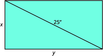 |
| Area is \(300\) square inches. | |
| Translate the information into a system of equations. | The diagonal of the right triangle is \(25\) inches. |
 |
|
| The area of the rectangle is \(300\) square inches. | |
 |
|
| Solve the system using substitution. |  |
| Solve the second equation for \(x\). |  |
| Substitute \(x\) into the first equation. |  |
 |
|
| Simplify. |  |
| Multiply by \(y^{2}\) to clear the fractions. |  |
| Put in standard form. |  |
| Solve by factoring. |  |
 |
|
 |
|
| Since \(y\) is a side of the rectangle, we discard the negative values. |  |
| Substitute back into the second equation. |  |
 |
|
| If the length is \(15\) inches, the width is \(20\) inches. | |
| If the length is \(20\) inches, the width is \(15\) inches. |
Edgar purchased a small \(20\)” TV for his garage. The size of a TV is measured on the diagonal of the screen. The screen also has an area of \(192\) square inches. What are the length and width of the TV screen?
- Answer
-
If the length is \(12\) inches, the width is \(16\) inches. If the length is \(16\) inches, the width is \(12\) inches.
The Harper family purchased a small microwave for their family room. The diagonal of the door measures \(15\) inches. The door also has an area of \(108\) square inches. What are the length and width of the microwave door?
- Answer
-
If the length is \(12\) inches, the width is \(9\) inches. If the length is \(9\) inches, the width is \(12\) inches.
Access these online resources for additional instructions and practice with solving nonlinear equations.
- Nonlinear Systems of Equations
- Solve a System of Nonlinear Equations
- Solve a System of Nonlinear Equations by Elimination
- System of Nonlinear Equations – Area and Perimeter Application
Key Concepts
- How to solve a system of nonlinear equations by graphing.
- Identify the graph of each equation. Sketch the possible options for intersection.
- Graph the first equation.
- Graph the second equation on the same rectangular coordinate system.
- Determine whether the graphs intersect.
- Identify the points of intersection.
- Check that each ordered pair is a solution to both original equations.
- How to solve a system of nonlinear equations by substitution.
- Identify the graph of each equation. Sketch the possible options for intersection.
- Solve one of the equations for either variable.
- Substitute the expression from Step 2 into the other equation.
- Solve the resulting equation.
- Substitute each solution in Step 4 into one of the original equations to find the other variable.
- Write each solution as an ordered pair.
- Check that each ordered pair is a solution to both original equations.
- How to solve a system of equations by elimination.
- Identify the graph of each equation. Sketch the possible options for intersection.
- Write both equations in standard form.
- Make the coefficients of one variable opposites.
Decide which variable you will eliminate.
Multiply one or both equations so that the coefficients of that variable are opposites. - Add the equations resulting from Step 3 to eliminate one variable.
- Solve for the remaining variable.
- Substitute each solution from Step 5 into one of the original equations. Then solve for the other variable.
- Write each solution as an ordered pair.
- Check that each ordered pair is a solution to both original equations.


