4.2: THE MEAN VALUE THEOREM

In this section, we focus on the Mean Value Theorem, one of the most important tools of calculus and one of the most beautiful results of mathematical analysis. The Mean Value Theorem we study in this section was stated by the French mathematician Augustin Louis Cauchy (1789-1857), which follows form a simpler version called Rolle's Theorem.

An important application of differentiation is solving optimization problems. A simple method for identifying local extrema of a function was found by the French mathematician Pierre de Fermat (1601-1665). Fermat's method can also be used to prove Rolle's Theorem.

We start with some basic definitions of minima and maxima. Recall that for \(a \in \mathbb{R}\) and \(\delta > 0\), the sets \(B(a ; \delta)\), \(B_{+}(a ; \delta)\), and \(B_{-}(a ; \delta)\) denote the intervals \((a-\delta, a+\delta)\), \((a, a+\delta)\) and \((a-\delta, a)\), respectively.

Definition \(\PageIndex{1}\)

Let \(D\) be a nonempty subset of \(\mathbb{R}\) and let \(f: D \rightarrow \mathbb{R}\). We say that \(f\) has a local (or relative) minimum at \(a \in D\) if there exists \(\delta > 0\) such that

\[f(x) \geq f(a) \text { for all } x \in B(a ; \delta) \cap D.\]

Similarly, we say that \(f\) has a local (or relative) maximum at \(a \in D\) if there exists \(\delta > 0\) such that

\[f(x) \leq f(a) \text { for all } x \in B(a ; \delta) \cap D .\]

In January 1638, Pierre de Fermat described his method for finding maxima and minima in a letter written to Marin Mersenne (1588-1648) who was considered as "the center of the world of science and mathematics during the first half of the 1600s." His method presented in the theorem below is now known as Fermat's Rule.

Theorem \(\PageIndex{1}\) - Fermat's Rule.

Let \(I\) be an open interval and \(f: I \rightarrow \mathbb{R}\). If \(f\) has a local minimum or maximum at \(a \in I\) and \(f\) is differentiable at \(a\), then \(f^{\prime}(a)=0\).

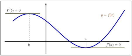
Figure \(4.1\): Illustration of Fermat's Rule.

Proof

Suppose \(f\) has a local minimum at \(a\). Then there exists \(\delta > 0\) sufficiently small such that

\[f(x) \geq f(a) \text { for all } x \in B(a ; \delta).\]

Since \(B_{+}(a ; \delta)\) is a subset of \(B(a ; \delta)\), we have

\[\frac{f(x)-f(a)}{x-a} \geq 0 \text { for all } x \in B_{+}(a ; \delta).\]

Taking into account the differentiability of \(f\) at \(a\) yields

\[f^{\prime}(a)=\lim _{x \rightarrow a} \frac{f(x)-f(a)}{x-a}=\lim _{x \rightarrow a^{+}} \frac{f(x)-f(a)}{x-a} \geq 0 .\]

Similarly,

\[\frac{f(x)-f(a)}{x-a} \leq 0 \text { for all } x \in B_{-}(a ; \delta)\].

It follows that

\[f^{\prime}(a)=\lim _{x \rightarrow a} \frac{f(x)-f(a)}{x-a}=\lim _{x \rightarrow a^{-}} \frac{f(x)-f(a)}{x-a} \leq 0 .\]

Therefore, \(f^{\prime}(a)=0\). The proof is similar for the case where \(f\) has a local maximum at \(a\). \(\square\)

Theorem \(\PageIndex{2}\) - Rolle's Theorem.

Let \(a,b \in \mathbb{R}\) with \(a < b\) and \(f:[a, b] \rightarrow \mathbb{R}\). Suppose \(f\) is continuous on \([a,b]\) and differentiable on \((a,b)\) with \(f(a)=f(b)\). Then there exists \(c \in (a,b)\) such that

\[f^{\prime}(c)=0 .\]

Proof

Since \(f\) is continuous on the compact \([a,b]\), by the extreme value theorem (Theorem 3.4.2) there exists \(\bar{x}_{1} \in[a, b]\) and \(\bar{x}_{2} \in[a, b]\) such that

\[f\left(\bar{x}_{1}\right)=\min \{f(x): x \in[a, b]\} \text { and } f\left(\bar{x}_{2}\right)=\max \{f(x): x \in[a, b]\} .\]

Then

\[f\left(\bar{x}_{1}\right) \leq f(x) \leq f\left(\bar{x}_{2}\right) \text { for all } x \in[a, b] .\]

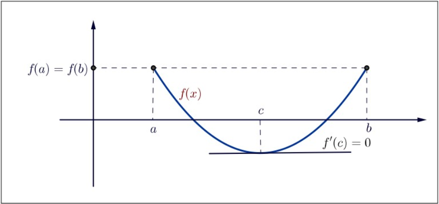
Figure \(4.2\): Illustration of Rolle's Theorem.

If \(\bar{x}_{1} \in(a, b)\) or \(\bar{x}_{2} \in(a, b)\), then \(f\) has a local minimum at \(\bar{x}_{1}\) or \(f\) has a local maximum at \(\bar{x}_{2}\). By Theorem 4.2.1, \(f^{\prime}\left(\bar{x}_{1}\right)=0\) or \(f^{\prime}\left(\bar{x}_{2}\right)=0\), and (4.3) holds with \(c = \bar{x}_{1}\) or \(c = \bar{x}_{2}\).

If both \(\bar{x}_{1}\) and \(\bar{x}_{2}\) are the endpoints of \([a,b]\), then \(f\left(\bar{x}_{1}\right)=f\left(\bar{x}_{2}\right)\) because \(f(a)=f(b)\). By (4.4), \(f\) is a constant function, so \(f^{\prime}(c)=0\) for any \(c \in (a,b)\). \(\square\)

We are now ready to use Rolle's Theorem to prove the Mean Value Theorem presented below.

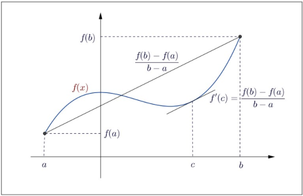
Figure \(4.3\): Illustration of the Mean Value Theorem.

Theorem \(\PageIndex{3}\) - Mean Value Theorem.

Let \(a,b \in \mathbb{R}\) with \(a < b\) and \(f:[a, b] \rightarrow \mathbb{R}\). Suppose \(f\) is continuous on \([a,b]\) and differentiable on \((a,b)\). Then there exists \(c \in (a,b)\) such that

\[f^{\prime}(c)=\frac{f(b)-f(a)}{b-a} .\]

Proof

The linear function whose graph goes through \((a, f(a))\) and \((b, f(b))\) is

\[g(x)=\frac{f(b)-f(a)}{b-a}(x-a)+f(a) .\]

Define

\[h(x)=f(x)-g(x)=f(x)-\left[\frac{f(b)-f(a)}{b-a}(x-a)+f(a)\right] \text { for } x \in[a, b] . \]

Then \(h(a) = h(b)\), and \(h\) satisfies the assumptions of Theorem 4.2.2. Thus, there exists \(c \in (a,b)\) such that \(h^{\prime}(c)=0\). Since

\[h^{\prime}(x)=f^{\prime}(x)-\frac{f(b)-f(a)}{b-a} ,\]

it follows that

\[f^{\prime}(c)-\frac{f(b)-f(a)}{b-a}=0 .\]

Thus, (4.5) holds. \(\square\)

Example \(\PageIndex{1}\)

We show that \(|\sin x| \leq|x|\) for all \(x \in \mathbb{R}\).

Solution

Let \(f(x)=\sin x\) for all \(x \in \mathbb{R}\). Then \(f^{\prime}(x) = \cos x\). Now, fix \(x \in \mathbb{R}\), \(x > 0\). By the Mean value Theorem applied to \(f\) on the interval \([0,x]\), there exists \(c \in (0,x)\) such that

\[\frac{\sin x-\sin 0}{x-0}=\cos c .\]

Therefore, \(\frac{|\sin x|}{|x|}=|\cos c|\). Since \(|\cos c| \leq 1\) we conclude \(|\sin x| \leq|x|\) for all \(x > 0\). Next suppose \(x < 0\). Another application of the Mean Value Theorem shows there exists \(c \in (x,0)\) such that

\[\frac{\sin 0-\sin x}{0-x}=\cos c .\]

Then, again, \(\frac{|\sin x|}{|x|}=|\cos c| \leq 1\). It follows that \(|\sin x| \leq|x|\) for \(x < 0\). Since equality holds for \(x = 0\), we conclude that \(|\sin x| \leq|x|\) for all \(x \in \mathbb{R}\).

Example \(\PageIndex{2}\)

We show that \(\sqrt{1+4 x}<(5+2 x) / 3\) for all \(x > 2\).

Solution

Let \(f(x)=\sqrt{1+4 x}\) for all \(x \geq 2\). Then

\[f^{\prime}(x)=\frac{4}{2 \sqrt{1+4 x}}=\frac{2}{\sqrt{1+4 x}} .\]

Now, fix \(x \in \mathbb{R}\) such that \(x > 2\). We apply the Mean Value Theorem to \(f\) on the interval \([2,x]\). Then, since \(f(2) = 3\), there exists \(c \in (2,x)\) such that

\[\sqrt{1+4 x}-3=f^{\prime}(c)(x-2) .\]

Since \(f^{\prime}(2)=2 / 3\) and \(f^{\prime}(c)<f^{\prime}(2)\) for \(c > 2\) we conclude that

\[\sqrt{1+4 x}-3<\frac{2}{3}(x-2) .\]

Rearranging terms provides the desired inequality.

A more general result which follows directly from the Mean Value Theorem is known as Cauchy's Theorem.

Theorem \(\PageIndex{4}\) - Cauchy's Theorem.

Let \(a,b \in \mathbb{R}\) with \(a < b\). Suppose \(f\) and \(g\) are continuous on \([a,b]\) and differentiable on \((a,b)\). Then there exists \(c \in (a,b)\) such that

\[[f(b)-f(a)] g^{\prime}(c)=[g(b)-g(a)] f^{\prime}(c).\]

Proof

Define

\[h(x)=[f(b)-f(a)] g(x)-[g(b)-g(a)] f(x) \text { for } x \in[a, b].\]

Then \(h(a)=f(b) g(a)-f(a) g(b)=h(b)\), and \(h\) satisfies the assumptions of Theorem 4.2.2. Thus, there exists \(c \in (a,b)\) such that \(h^{\prime}(c)=0\). Since

\[h^{\prime}(x)=[f(b)-f(a)] g^{\prime}(x)-[g(b)-g(a)] f^{\prime}(x),\]

this implies (4.6). \(\square\)

The following theorem shows that the derivative of a differentiable function on \([a,b]\) satisfies the intermediate value property although the derivative function is not assumed to be continuous. To give the theorem in its greatest generality, we introduce a couple of definitions.

Definition \(\PageIndex{2}\)

Let \(a,b \in \mathbb{R}\), \(a < b\), and \(f: [a,b] \rightarrow \mathbb{R}\). If the limit

\[\lim _{x \rightarrow a^{+}} \frac{f(x)-f(a)}{x-a}\]

exists, we say that \(f\) has a right derivative at \(a\) and write

\[f_{+}^{\prime}(a)=\lim _{x \rightarrow a^{+}} \frac{f(x)-f(a)}{x-a}.\]

If the limit

\[\lim _{x \rightarrow b^{-}} \frac{f(x)-f(b)}{x-b}\]

exists, we say that \(f\) has a left derivative at \(b\) and write

\[f_{-}^{\prime}(b)=\lim _{x \rightarrow b^{-}} \frac{f(x)-f(b)}{x-b}.\]

We will say that \(f\) is differentiable on \([a,b]\) if \(f^{\prime}(x)\) exists for each \(x \in (a,b)\) and, in addition, both \(f_{+}^{\prime}(a)\) and \(f_{-}^{\prime}(b)\) exist.

Theorem \(\PageIndex{5}\) - Intermediate Value Theorem for Derivatives.

Let \(a,b \in \mathbb{R}\) with \(a < b\). Suppose \(f\) is differentiable on \([a,b]\) and

\[f_{+}^{\prime}(a)<\lambda<f_{-}^{\prime}(b).\]

Then there exists \(c \in (a,b)\) such that

\[f^{\prime}(c)=\lambda.\]

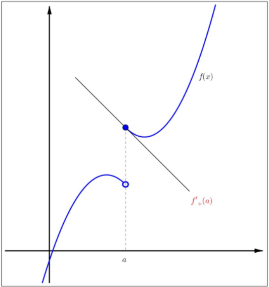
Figure \(4.4\): Right derivative.

Proof

Define the function \(g: [a,b] \rightarrow \mathbb{R}\) by

\[g(x)=f(x)-\lambda x.\]

Then \(g\) is differentiable on \([a,b]\) and

\[g_{+}^{\prime}(a)<0<g_{-}^{\prime}(b).\]

Thus,

\[\lim _{x \rightarrow a^{+}} \frac{g(x)-g(a)}{x-a}<0.\]

It follows that there exists \(\delta_{1} > 0\) such that

\[g(x)<g(a) \text { for all } x \in\left(a, a+\delta_{1}\right) \cap[a, b].\]

SImilarly, there exists \(\delta_{2} > 0\) such that

\[g(x)<g(b) \text { for all } x \in\left(b-\delta_{2}, b\right) \cap[a, b].\]

Since \(g\) is continuous on \([a,b]\), it attains its minimum at a point \(c \in [a,b]\). From the observations above, it follows that \(c \in (a,b)\). This implies \(g^{\prime}(c)=0\) or, equivalently, that \(f^{\prime}(c)=\lambda\). \(square\)

Remark \(\PageIndex{6}\)

The same conclusion follows if \(f_{+}^{\prime}(a)>\lambda>f_{-}^{\prime}(b)\).

Exercise \(\PageIndex{1}\)

Let \(f\) and \(g\) be differentiable at \(x_{0}\). Suppose \(\) and

\[f(x) \leq g(x) \text { for all } x \in \mathbb{R}.\]

Prove that \(f^{\prime}\left(x_{0}\right)=g^{\prime}\left(x_{0}\right)\).

Answer

Add texts here. Do not delete this text first.

Exercise \(\PageIndex{2}\)

Prove the following inequalities using the Mean Value Theorem.

1. \(\sqrt{1+x}<1+\frac{1}{2} x \text { for } x>0\).
2. \(e^{x}>1+x\), for \(x > 0\). (Assume known that the derivative of \(e^{x}\) is itself.)
3. \(\frac{x-1}{x}<\ln x<x-1, \text { for } x>1\). (Assume known that the derivative of \(\ln x\) is \(1 / x\).)

Answer

Add texts here. Do not delete this text first.

Exercise \(\PageIndex{3}\)

Prove that \(|\sin (x)-\sin (y)| \leq|x-y|\) for all \(x,y \in \mathbb{R}\).

Answer

Add texts here. Do not delete this text first.

Exercise \(\PageIndex{4}\)

Let \(n\) be a positive integer and let \(a_{k}, b_{k} \in \mathbb{R}\) for \(k=1, \ldots, n\). Prove that the equation

\[x+\sum_{k=1}^{n}\left(a_{k} \sin k x+b_{k} \cos k x\right)=0\]

has a solution on \((-\pi, \pi)\).

Answer

Add texts here. Do not delete this text first.

Exercise \(\PageIndex{5}\)

Let \(f\) and \(g\) be differentiable functions on \([a,b]\). Suppose \(g(x) \neq 0\) and \(g^{\prime}(x) \neq 0\) for all \(x \in [a,b]\). Prove that there exists \(c \in (a,b)\) such that

\[\frac{1}{g(b)-g(a)} \mid \begin{array}{ll}
f(a) & f(b) \\
g(a) & g(b)
\end{array} \mid=\frac{1}{g^{\prime}(c)} \mid \begin{array}{cc}
f(c) & g(c) \\
f^{\prime}(c) & g^{\prime}(c)
\end{array} \mid ,\]

where the bars denote determinants of the two-by-two matrices.

Answer

Add texts here. Do not delete this text first.

Exercise \(\PageIndex{6}\)

Let \(n\) be a fixed positive integer.

1. Suppose \(a_{1}, a_{2}, \ldots, a_{n}\) satisfy

\[a_{1}+\frac{a_{2}}{2}+\cdots+\frac{a_{n}}{n}=0.\]

Prove that the equation

\[a_{1}+a_{2} x+a_{3} x^{2}+\cdots+a_{n} x^{n-1}=0\]

has a solution in \((0,1)\).

2. Suppose \(a_{0}, a_{1}, \ldots, a_{n}\) satisfy

\[\sum_{k=0}^{n} \frac{a_{k}}{2 k+1}=0.\]

Prove that the equation

\[\sum_{k=0}^{n} a_{k} \cos (2 k+1) x=0\]

has a solution on \(\left(0, \frac{\pi}{2}\right)\).

Answer

Add texts here. Do not delete this text first.

Exercise \(\PageIndex{7}\)

Let \(f:[0, \infty) \rightarrow \mathbb{R}\) be a differentiable function. Prove that if both \(\lim _{x \rightarrow \infty} f(x)\) and \(\lim _{x \rightarrow \infty} f^{\prime}(x)\) exist, then \(\lim _{x \rightarrow \infty} f^{\prime}(x)=0\)

Answer

Add texts here. Do not delete this text first.

Exercise \(\PageIndex{8}\)

Let \(f:[0, \infty) \rightarrow \mathbb{R}\) be a differentiable function.

1. Show that if \(\lim _{x \rightarrow \infty} f^{\prime}(x)=a\), then \(\lim _{x \rightarrow \infty} \frac{f(x)}{x}=a\).
2. Show that if \(\lim _{x \rightarrow \infty} f^{\prime}(x)=\infty\), then \(\lim _{x \rightarrow \infty} \frac{f(x)}{x}=\infty\).
3. Are the converses in part (a) and part (b) true?

Answer

Add texts here. Do not delete this text first.