3.4: Complex Numbers

With all the operations defined in §§1-3, \(E^{n}(n>1)\) is not yet a field because of the lack of a vector multiplication satisfying the field axioms. We shall now define such a multiplication, but only for \(E^{2} .\) Thus \(E^{2}\) will become a field, which we shall call the complex field, \(C .\)

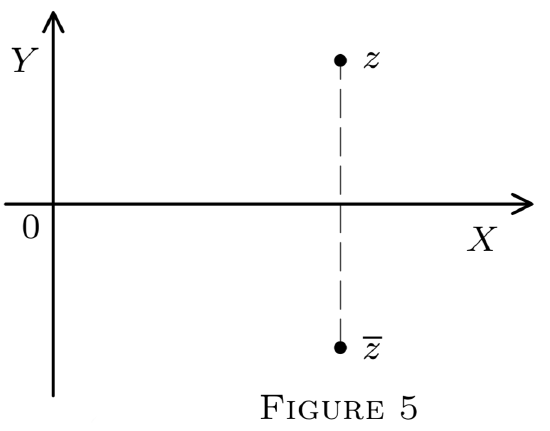
We make some changes in notation and terminology here. Points of\(E^{2},\) when regarded as elements of \(C,\) will be called complex numbers (each being an ordered pair of real numbers). We denote them by single letters (preferably z) without a bar or an arrow. For example, \(z=(x, y)\). We preferably write \((x, y)\) for \(\left(x_{1}, x_{2}\right) .\) If \(z=(x, y),\) then \(x\) and \(y\) are called the real and imaginary parts of \(z,\) respectively, \(^{1}\) and \(\overline{z}\) denotes the complex number \((x,-y),\) called the conjugate of \(z\) (see Figure 5\()\).

Complex numbers with vanishing imaginary part, \((x, 0),\) are called real points of \(C .\) For brevity, we simply write \(x\) for \((x, 0) ;\) for example, \(2=(2,0)\). In particular, \(1=(1,0)=\overline{\theta}_{1}\) is called the real unit in \(C .\) Points with vanishing real part, \((0, y),\) are called (purely) imaginary numbers. In particular, \(\overline{\theta}_{2}=(0,1)\) is such a number; we shall now denote it by \(i\) and call it the imaginary unit in \(C .\) Apart from these peculiarities, all our former definitions of §§1-3 remain valid in \(E^{2}=C .\) In particular, if \(z=(x, y)\) and \(z^{\prime}=\left(x^{\prime}, y^{\prime}\right),\) we have

\[z \pm z^{\prime}=(x, y) \pm\left(x^{\prime}, y^{\prime}\right)=\left(x \pm x^{\prime}, y \pm y^{\prime}\right),\]

\[\rho\left(z, z^{\prime}\right)=\sqrt{\left(x-x^{\prime}\right)^{2}+\left(y-y^{\prime}\right)^{2}}, \text{ and} \]

\[|z|=\sqrt{x^{2}+y^{2}}.\]

All theorems of §§1-3 are valid.

We now define the new multiplication in \(C,\) which will make it a field.

Definition

\[\text{If } z=(x, y) \text{ and } z^{\prime}=\left(x^{\prime}, y^{\prime}\right), \text{ then } z z^{\prime}=\left(x x^{\prime}-y y^{\prime}, x y^{\prime}+y x^{\prime}\right).\]

Theorem \(\PageIndex{1}\)

\(E^{2}=C\) is a field, with zero element \(0=(0,0)\) and unity \(1=(1, 0)\), under addition and multiplication as defined above.

Proof

We only must show that multiplication obeys Axioms 1-6 of the field axioms. Note that for addition, all is proved in Theorem 1 of §§1-3.

Axiom 1 (closure) is obvious from our definition, for if \(z\) and \(z^{\prime}\) are in \(C,\) so is \(z z^{\prime}\).

To prove commutativity, take any complex numbers

\[z=(x, y) \text{ and } z^{\prime}=\left(x^{\prime}, y^{\prime}\right)\]

and verify that \(z z^{\prime}=z^{\prime} z .\) Indeed, by definition,

\[z z^{\prime}=\left(x x^{\prime}-y y^{\prime}, x y^{\prime}+y x^{\prime}\right) \text{ and } z^{\prime} z=\left(x^{\prime} x-y^{\prime} y, x^{\prime} y+y^{\prime} x\right);\]

but the two expressions coincide by the commutative laws for real numbers. Associativity and distributivity are proved in a similar manner.

Next, we show that \(1=(1,0)\) satisfies Axiom 4(b), i.e., that \(1 z=z\) for any complex number \(z=(x, y) .\) In fact, by definition, and by axioms for \(E^{1}\),

\[1 z=(1,0)(x, y)=(1 x-0 y, 1 y+0 x)=(x-0, y+0)=(x, y)=z.\]

It remains to verify Axiom 5(b), i.e., to show that each complex number \(z=(x, y) \neq(0,0)\) has an inverse \(z^{-1}\) such that \(z z^{-1}=1 .\) It turns out that the inverse is obtained by setting

\[z^{-1}=\left(\frac{x}{|z|^{2}},-\frac{y}{|z|^{2}}\right).\]

In fact, we then get

\[z z^{-1}=\left(\frac{x^{2}}{|z|^{2}}+\frac{y^{2}}{|z|^{2}},-\frac{x y}{|z|^{2}}+\frac{y x}{|z|^{2}}\right)=\left(\frac{x^{2}+y^{2}}{|z|^{2}}, 0\right)=(1,0)=1\]

since \(x^{2}+y^{2}=|z|^{2},\) by definition. This completes the proof. \(\square\)

corollary \(\PageIndex{1}\)

\(i^{2}=-1 ; i . e .,(0,1)(0,1)=(-1,0)\).

Proof

By definition, \((0,1)(0,1)=(0 \cdot 0-1 \cdot 1,0 \cdot 1+1 \cdot 0)=(-1,0)\).

Thus \(C\) has an element \(i\) whose square is \(-1,\) while \(E^{1}\) has no such element, by Corollary 2 in Chapter \(2,8\{1-4 .\) This is no contradiction since that corollary holds in ordered fields only. It only shows that \(C\) cannot be made an ordered field.

However, the "real points" in \(C\) form a subfield that can be ordered by setting

\[(x, 0)<\left(x^{\prime}, 0\right) \text{ iff } x<x^{\prime} \text{ in } E^{1} .\]

Then this subfield behaves exactly like \(E^{1} .\) Therefore, it is customary not to distinguish between "real points in \(C^{\prime \prime}\) and "real numbers," identifying \((x, 0)\) with \(x .\) With this convention, \(E^{1}\) simply is a subset \((\)and a subfield \()\) of \(C .\) Henceforth, we shall simply say that "x is real" or "x \(\in E^{1 \prime}\) instead of "\(x =(x, 0)\) is a real point." We then obtain the following result.

Theorem \(\PageIndex{2}\)

Every \(z \in C\) has a unique representation as

\[z=x+y i,\]

where \(x\) and \(y\) are real and \(i=(0,1) .\) Specifically,

\[z=x+y i \text{ iff } z=(x, y).\]

Proof

By our conventions, \(x=(x, 0)\) and \(y=(y, 0),\) so

\[x+y i=(x, 0)+(y, 0)(0,1).\]

Computing the right-hand expression from definitions, we have for any \(x, y \in E^{1}\) that

\[x+y i=(x, 0)+(y \cdot 0-0 \cdot 1, y \cdot 1+0 \cdot 1)=(x, 0)+(0, y)=(x, y).\]

Thus \((x, y)=x+y i\) for any \(x, y \in E^{1} .\) In particular, if \((x, y)\) is the given number \(z \in C\) of the theorem, we obtain \(z=(x, y)=x+y i,\) as required.

To prove uniqueness, suppose that we also have

\[z=x^{\prime}+y^{\prime} i \text{ with } x^{\prime}=\left(x^{\prime}, 0\right) \text{ and } y^{\prime}=\left(y^{\prime}, 0\right).\]

Then, as shown above, \(z=\left(x^{\prime}, y^{\prime}\right) .\) since also \(z=(x, y),\) we have \((x, y)= \left(x^{\prime}, y^{\prime}\right),\) i.e., the two ordered pairs coincide, and so \(x=x^{\prime}\) and \(y=y^{\prime}\) after all. \(\square\)

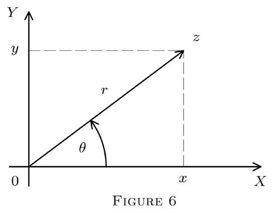
Geometrically, instead of Cartesian coordinates \((x, y),\) we may also use polar coordinates \(r, \theta,\) where

\[r=\sqrt{x^{2}+y^{2}}=|z|\]

and \(\theta\) is the (counterclockwise) rotation angle from the \(x\)-axis to the directed line \(\overrightarrow{0 z} ;\) see Figure \(6 .\) Clearly, \(z\) is uniquely determined by \(r\) and \(\theta\) but \(\theta\) is not uniquely determined by \(z ;\) indeed, the same point of \(E^{2}\) results if \(\theta\) is replaced by \(\theta+2 n \pi(n=1,2, \ldots)\). (If \(z=0,\) then \(\theta\) is not defined at all.) The values \(r\) and \(\theta\) are called, respectively, the modulus and argument of \(z=(x, y) .\) By elementary trigonometry, \(x=r \cos \theta\) and \(y=r \sin \theta .\) Substituting in \(z=x+y i,\) we obtain the following corollary.

corollary \(\PageIndex{2}\)

\[z=r(\cos \theta+i \sin \theta)(\text{trigonometric or polar form of }z).\]