
13.3: Amortization Schedules
- Page ID
- 22147

\( \newcommand{\vecs}[1]{\overset { \scriptstyle \rightharpoonup} {\mathbf{#1}} } \)
\( \newcommand{\vecd}[1]{\overset{-\!-\!\rightharpoonup}{\vphantom{a}\smash {#1}}} \)
\( \newcommand{\id}{\mathrm{id}}\) \( \newcommand{\Span}{\mathrm{span}}\)
( \newcommand{\kernel}{\mathrm{null}\,}\) \( \newcommand{\range}{\mathrm{range}\,}\)
\( \newcommand{\RealPart}{\mathrm{Re}}\) \( \newcommand{\ImaginaryPart}{\mathrm{Im}}\)
\( \newcommand{\Argument}{\mathrm{Arg}}\) \( \newcommand{\norm}[1]{\| #1 \|}\)
\( \newcommand{\inner}[2]{\langle #1, #2 \rangle}\)
\( \newcommand{\Span}{\mathrm{span}}\)
\( \newcommand{\id}{\mathrm{id}}\)
\( \newcommand{\Span}{\mathrm{span}}\)
\( \newcommand{\kernel}{\mathrm{null}\,}\)
\( \newcommand{\range}{\mathrm{range}\,}\)
\( \newcommand{\RealPart}{\mathrm{Re}}\)
\( \newcommand{\ImaginaryPart}{\mathrm{Im}}\)
\( \newcommand{\Argument}{\mathrm{Arg}}\)
\( \newcommand{\norm}[1]{\| #1 \|}\)
\( \newcommand{\inner}[2]{\langle #1, #2 \rangle}\)
\( \newcommand{\Span}{\mathrm{span}}\) \( \newcommand{\AA}{\unicode[.8,0]{x212B}}\)
\( \newcommand{\vectorA}[1]{\vec{#1}} % arrow\)
\( \newcommand{\vectorAt}[1]{\vec{\text{#1}}} % arrow\)
\( \newcommand{\vectorB}[1]{\overset { \scriptstyle \rightharpoonup} {\mathbf{#1}} } \)
\( \newcommand{\vectorC}[1]{\textbf{#1}} \)
\( \newcommand{\vectorD}[1]{\overrightarrow{#1}} \)
\( \newcommand{\vectorDt}[1]{\overrightarrow{\text{#1}}} \)
\( \newcommand{\vectE}[1]{\overset{-\!-\!\rightharpoonup}{\vphantom{a}\smash{\mathbf {#1}}}} \)
\( \newcommand{\vecs}[1]{\overset { \scriptstyle \rightharpoonup} {\mathbf{#1}} } \)
\( \newcommand{\vecd}[1]{\overset{-\!-\!\rightharpoonup}{\vphantom{a}\smash {#1}}} \)
\(\newcommand{\avec}{\mathbf a}\) \(\newcommand{\bvec}{\mathbf b}\) \(\newcommand{\cvec}{\mathbf c}\) \(\newcommand{\dvec}{\mathbf d}\) \(\newcommand{\dtil}{\widetilde{\mathbf d}}\) \(\newcommand{\evec}{\mathbf e}\) \(\newcommand{\fvec}{\mathbf f}\) \(\newcommand{\nvec}{\mathbf n}\) \(\newcommand{\pvec}{\mathbf p}\) \(\newcommand{\qvec}{\mathbf q}\) \(\newcommand{\svec}{\mathbf s}\) \(\newcommand{\tvec}{\mathbf t}\) \(\newcommand{\uvec}{\mathbf u}\) \(\newcommand{\vvec}{\mathbf v}\) \(\newcommand{\wvec}{\mathbf w}\) \(\newcommand{\xvec}{\mathbf x}\) \(\newcommand{\yvec}{\mathbf y}\) \(\newcommand{\zvec}{\mathbf z}\) \(\newcommand{\rvec}{\mathbf r}\) \(\newcommand{\mvec}{\mathbf m}\) \(\newcommand{\zerovec}{\mathbf 0}\) \(\newcommand{\onevec}{\mathbf 1}\) \(\newcommand{\real}{\mathbb R}\) \(\newcommand{\twovec}[2]{\left[\begin{array}{r}#1 \\ #2 \end{array}\right]}\) \(\newcommand{\ctwovec}[2]{\left[\begin{array}{c}#1 \\ #2 \end{array}\right]}\) \(\newcommand{\threevec}[3]{\left[\begin{array}{r}#1 \\ #2 \\ #3 \end{array}\right]}\) \(\newcommand{\cthreevec}[3]{\left[\begin{array}{c}#1 \\ #2 \\ #3 \end{array}\right]}\) \(\newcommand{\fourvec}[4]{\left[\begin{array}{r}#1 \\ #2 \\ #3 \\ #4 \end{array}\right]}\) \(\newcommand{\cfourvec}[4]{\left[\begin{array}{c}#1 \\ #2 \\ #3 \\ #4 \end{array}\right]}\) \(\newcommand{\fivevec}[5]{\left[\begin{array}{r}#1 \\ #2 \\ #3 \\ #4 \\ #5 \\ \end{array}\right]}\) \(\newcommand{\cfivevec}[5]{\left[\begin{array}{c}#1 \\ #2 \\ #3 \\ #4 \\ #5 \\ \end{array}\right]}\) \(\newcommand{\mattwo}[4]{\left[\begin{array}{rr}#1 \amp #2 \\ #3 \amp #4 \\ \end{array}\right]}\) \(\newcommand{\laspan}[1]{\text{Span}\{#1\}}\) \(\newcommand{\bcal}{\cal B}\) \(\newcommand{\ccal}{\cal C}\) \(\newcommand{\scal}{\cal S}\) \(\newcommand{\wcal}{\cal W}\) \(\newcommand{\ecal}{\cal E}\) \(\newcommand{\coords}[2]{\left\{#1\right\}_{#2}}\) \(\newcommand{\gray}[1]{\color{gray}{#1}}\) \(\newcommand{\lgray}[1]{\color{lightgray}{#1}}\) \(\newcommand{\rank}{\operatorname{rank}}\) \(\newcommand{\row}{\text{Row}}\) \(\newcommand{\col}{\text{Col}}\) \(\renewcommand{\row}{\text{Row}}\) \(\newcommand{\nul}{\text{Nul}}\) \(\newcommand{\var}{\text{Var}}\) \(\newcommand{\corr}{\text{corr}}\) \(\newcommand{\len}[1]{\left|#1\right|}\) \(\newcommand{\bbar}{\overline{\bvec}}\) \(\newcommand{\bhat}{\widehat{\bvec}}\) \(\newcommand{\bperp}{\bvec^\perp}\) \(\newcommand{\xhat}{\widehat{\xvec}}\) \(\newcommand{\vhat}{\widehat{\vvec}}\) \(\newcommand{\uhat}{\widehat{\uvec}}\) \(\newcommand{\what}{\widehat{\wvec}}\) \(\newcommand{\Sighat}{\widehat{\Sigma}}\) \(\newcommand{\lt}{<}\) \(\newcommand{\gt}{>}\) \(\newcommand{\amp}{&}\) \(\definecolor{fillinmathshade}{gray}{0.9}\)In the previous two sections, you have been working on parts of an entire puzzle. You have calculated the interest and principal portions for either a single payment or a series of payments. Additionally, you calculated the final payment amount along with its principal and interest components. The next task is to put these concepts together into a complete understanding of amortization. This involves developing a complete amortization schedule for an annuity (loan or investment annuity). Additionally, you will create partial amortization schedules that depict specific ranges of payments for a particular annuity.
These concepts primarily apply to accounting. Accountants must record debts properly on balance sheets, make proper journal entries into the accounting books, and track interest expenses clearly. Depreciation of fixed assets uses similar amortization processes and schedules. Bond premiums and discounts (discussed in Chapter 14) also use amortization.
On the personal side, these schedules help you understand any of your loans, mortgages, or investment annuities. Sometimes seeing the true amount of interest you are paying may motivate you to pay the debt off faster. Courts also use these schedules to settle legal matters such as alimony payments.
The Complete Amortization Schedule
An amortization schedule shows the payment amount, principal component, interest component, and remaining balance for every payment in the annuity. As the title suggests, it provides a complete understanding of where the money goes.
How It Works
| Payment Number | Payment Amount ($) (PMT) | Interest Portion ($) (INT) | Principal Portion ($) (PRN) | Principal Balance Remaining ($) (PRN) |
|---|---|---|---|---|
| 0–Start | N/A | N/A | N/A | (3) |
| 1 | (4) | (5) | (6) | (7) |
| etc. | ||||
| Last payment | (11) | (10) | (9) | $0.00 |
| Total | *if needed | (13) | *equals original loan balance | N/A |
Follow these steps to develop a complete amortization schedule:
Step 1: Identify all of the time value of money variables (\(N, IY, PV_{ORD}, PMT, FV, PY, CY\)). If either \(N\) or \(PMT\) is unknown, solve for it using an appropriate formula. Remember to round \(PMT\) to two decimals.
Step 2: Set up an amortization schedule template as per the table above. Cells of the table are marked with the step numbers that follow. The number of payment rows in the table equals the number of payments in the annuity.Note that in the instance of a general annuity, the table does not distinguish between earned interest and accrued interest. The schedule reflects only the total of earned interest and interest accrued at the time of a payment.
Step 3: On the first row, fill in the original principal of the annuity, or \(PV_{ORD}\).
Step 4: Fill in the rounded annuity payment (\(PMT\)) all the way down the column except for the final payment row.
Step 5: Calculate the interest portion of the current annuity payment using Formula 13.1. Round the number to two decimals for the table but retain the decimals for future calculations.
Step 6: Calculate the principal portion of the current annuity payment using Formula 13.2. The interest component is the un-rounded interest number from step 5. Round the result to two decimals for the table but retain the decimals for future calculations.
Step 7: Calculate the new principal balance remaining by taking the previous un-rounded balance on the line above and subtracting the un-rounded principal portion (PRN) of the current payment. This is Formula 13.3 rearranged such that \(BAL_{P2} = BAL_{P1} − PRN\). Round the result to two decimals for the table but retain the decimals for future calculations.
Step 8: Repeat steps 5 through 7 for each annuity payment until you reach the final payment.
Step 9: For the final payment, the principal portion is exactly equal to the previous balance remaining on the line above. Round the result to two decimals for the table but retain the decimals for future calculations. Enter "$0.00" in the Principal Balance Remaining.
Step 10: Calculate the interest portion of the final annuity payment using Formula 13.1. Round the result to two decimals for the table but retain the decimals for future calculations.
Step 11: Calculate the final payment by adding the un-rounded principal and interest portions of the final payment together. Round this number to two decimals.
Step 12: Since all numbers are rounded to two decimals throughout the table, check the table for the "missing penny," as discussed below. Always ensure that for each row the previous balance minus current principal equals the new balance. Then check that the principal portion plus interest portion equals the annuity payment amount. Make any penny adjustments as needed.
Step 13: Sum the interest portion column in the schedule. Note that no total is necessary for the principal portion since it equals the original principal of the annuity!
Important Notes
The "Missing Penny"
In the creation of the amortization schedule, you always round the numbers off to two decimals since you are dealing with currency. However, as per the rules of rounding, you do not round any numbers in your calculations until you reach the end of the amortization schedule and the annuity has been reduced to zero.
As a result, you have a triple rounding situation involving the balance along with the principal and interest components on every line of the table. What sometimes happens is that a "missing penny" occurs and the schedule needs to be corrected as per step 12 of the process above. In other words, calculations will sometimes appear to be off by a penny. You can identify the "missing penny" when one of the two standard calculations using the rounded numbers from the schedule becomes off by a penny:
1. Previous \(BAL − PRN =\) current \(BAL\) (step 7)
or
2. \(PMT − INT = PRN\) (step 6)
It is important to remember, though, that in actuality there is no "missing penny" in these calculations. It shows up only because you are rounding off numbers. If you were not rounding numbers, this "missing penny" would never occur.
In these instances of the "missing penny", you adjust the schedule as needed to ensure that the math works properly at all times. The golden rule, though, is that the balance in the account (\(BAL\)) is always correct and should NEVER be adjusted. Follow this order in making any adjustments:
- Adjust the \(PRN\) if necessary such that the previous \(BAL − PRN =\) current \(BAL\).
- Then adjust \(INT\) if necessary such that \(PMT − PRN = INT\).
Usually these adjustments come in pairs, meaning that if you need to adjust the \(PRN\) up by a penny, somewhere later in the schedule you will need to adjust the \(PRN\) down by a penny. Ultimately, these changes in most circumstances have no impact on the total interest (\(INT\)) or total principal (\(PRN\)) components, since the "missing penny" is nothing more than a rounding error within the schedule.
Your BAII Plus Calculator
The calculator speeds up the repetitive calculations required in the amortization schedule. To create the schedule using the calculator, adapt the steps as follows:
Step 1: Load the calculator with all seven time value of money variables, solving for any unknowns. Ensure that \(PMT\) is keyed in with two decimals, and obey the cash flow sign convention.
Steps 2–4: Unchanged.
Steps 5–7: Open the AMORT function. Set the P1 = 1 and P2 = 1. In the appropriate column, record the \(BAL\), \(PRN\), and \(INT\) rounded to two decimals.
Step 8: Repeat steps 5–7 by increasing the payment number (P1 and P2) by one each time. Ensure P1 = P2 at all times.
Step 9: Unchanged.
Step 10: Set the P1 and P2 to the final payment number. Record the \(INT\) amount.
Steps 11–12: Unchanged.
Step 13: Set the P1 = 1 and P2 = final payment number. Record the \(INT\) amount.
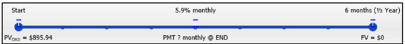
Tamara purchased a new dishwasher from The Bay for $895.94. By placing it on her Bay credit card, she can pay off the dishwasher through a special six-month payment plan promotion that charges her 5.9% compounded monthly. Construct the complete amortization schedule for Tamara and total her interest charges.
Solution
Construct a complete amortization schedule for the dishwasher payments along with the total interest paid.
What You Already Know
Step 1:
The timeline for Tamara's purchase appears in the timeline.
\(PV_{ORD}\) = $895.94, \(IY\) = 5.9%, \(CY\) = 12, \(PY\) = 12, Years = 0.5, \(FV\) = $0
How You Will Get There
Step 1 (continued):
Solve for the payment (\(PMT\)) using Formulas 9.1, 11.1, and 11.4.
Step 2:
Set up the amortization table.
Steps 3 and 4:
Fill in the original principal and payment column.
Steps 5 to 8:
For each line use Formula 13.1 and Formula 13.2 and the rearranged Formula 13.3.
Steps 9 to 11:
Fill in the principal and balance remaining, calculate the interest using Formula 13.1, and determine the final payment by adding the interest and principal components together.
Step 12:
Check for the "missing penny."
Step 13:
Sum the interest portion.
Perform
Step 1 (continued):
\(i=5.9 \% / 12=0.491 \overline{6} \% ; N=12 \times 1 / 2=6\) payments
\[\$ 895.94=PMT\left[\dfrac{1-\left[\dfrac{1}{(1+0.00491 \overline{6})^{\frac{12}{12}}}\right]^{6}}{(1+0.00491 \overline{6}) ^{\frac{12}{12}}-1}\right] \nonumber \]
\[PMT=\dfrac{\$ 895.94}{\left[\dfrac{1-0.971001}{0.00491 \overline{6}}\right]}=\dfrac{\$ 895.94}{[5.89808]}=\$ 151.90 \nonumber \]
Steps 2 to 11 (with some calculations) are detailed in the table below:
| Payment Number | Payment Amount ($) (PMT) | Interest Portion ($) (INT) | Principal Portion ($) (PRN) | Principal Balance Remaining ($) (PRN) |
|---|---|---|---|---|
| 0–Start | $895.94 | |||
| 1 | $151.90 | (1) $4.41 | (2) $147.49 | (3) $748.45 |
| 2 | $151.90 | $3.68 | $148.22 | $600.22 |
| 3 | $151.90 | $2.95 | $148.95 | $451.28 |
| 4 | $151.90 | $2.22 | $149.68 | $301.59 |
| 5 | $151.90 | $1.48 | $150.42 | $151.18 |
| 6 | (4) $151.90 | $0.74 | $151.18 | $0.00 |
| Total |
(1) \(INT =\$ 895.94 \times\left((1+0.00491 \overline{6})^{\frac{12}{12}}-1\right)=\$ 4.405038\)
(2) \(PRN=\$ 151.90-\$ 4.405038=\$ 147.494961\)
(3) \(BAL_{P2}=\$ 895.94-\$ 147.494961=\$ 748.445038 \)
(4) Final Payment \(=\$ 151.177613+\$ 0.742386=\$ 151.92\)
Steps 12 to 13: Adjust for the "missing pennies" (noted in red) and total the interest.
| Payment Number | Payment Amount ($) (PMT) | Interest Portion ($) (INT) | Principal Portion ($) (PRN) | Principal Balance Remaining ($) (PRN) |
|---|---|---|---|---|
| 0–Start | $895.94 | |||
| 1 | $151.90 | (1) $4.41 | (2) $147.49 | (3) $748.45 |
| 2 | $151.90 | $3.67 | $148.23 | $600.22 |
| 3 | $151.90 | $2.96 | $148.94 | $451.28 |
| 4 | $151.90 | $2.21 | $149.69 | $301.59 |
| 5 | $151.90 | $1.49 | $150.41 | $151.18 |
| 6 | (4) $151.90 | $0.74 | $151.18 | $0.00 |
| Total | $911.42 | $15.48 | $895.94 |
Calculator Instructions
| N | I/Y | PV | PMT | FV | P/Y | C/Y |
|---|---|---|---|---|---|---|
| 6 | 5.9 | 895.94 |
Answer: -151.903441 Re-keyed as: -151.90 |
0 | 12 | 12 |
| Payment | P1 | P2 | BAL (output) | PRN (output) | INT (output) |
|---|---|---|---|---|---|
| 1 | 1 | 1 | 748.4450383 | 147.494961 | 4.4050383 |
| 2 | 2 | 2 | 600.224893 | 148.22014 | 3.679854 |
| 3 | 3 | 3 | 451.275998 | 148.948894 | 2.951105 |
| 4 | 4 | 4 | 301.594772 | 149.681226 | 2.218773 |
| 5 | 5 | 5 | 151.177613 | 150.417159 | 1.482840 |
| 6 | 6 | 6 | 0.020903 | 151.156710 *add BAL=151.1777613 |
0.743289 |
| Total | 1 | 6 | 0.020903 | 895.919096 * add BAL=895.94 |
15.480903 |
The complete amortization schedule is shown in the table above. The total interest Tamara is to pay on her dishwasher is $15.48.
Amortization Schedule Due
In the instance of an annuity due, you require a small modification to the amortization schedule, as illustrated in the next table. Notice that the headers of the second and fifth columns have been modified to clarify the timing of the payment and point in time when the balance is achieved. Each line of the table still represents one payment interval.
| Payment Number | Payment Amount at Beginning of Interval ($) (PMT) | Interest Portion ($) (INT) | Principal Portion ($) (PRN) | Principal Balance Remaining at End of Interval($) (PRN) |
|---|---|---|---|---|
| 0–Start | N/A | N/A | N/A | (3) |
| 1 | (4) | (5) | (6) | (7) |
| etc. | ||||
| Last payment | (11) | $0.00 (10) | (9) | $0.00 |
| Total | *if needed | (13) | *equals original loan balance | N/A |
The Formula
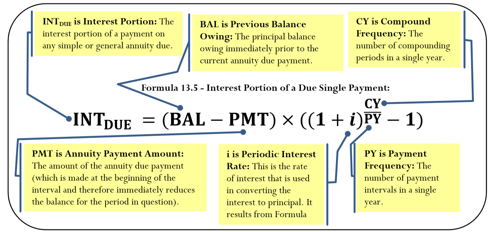
Be sure to determine any calculated amounts such as PMT through the appropriate annuity due formulas and not the ordinary annuity formulas. Recall that in an annuity the annuity payment is made at the beginning of the interval, which immediately reduces the balance eligible for interest. Calculating interest requires Formula 13.1 to be adapted and reintroduced as Formula 13.5.
How It Works
When you work with the amortization of annuities due, you must make the following modifications to the 13-step process:
Step 1: Ensure that you use appropriate annuity due formulas when solving for any unknown variable.
Step 5: Recall that the payment is made at the beginning of the interval, which immediately reduces the balance eligible for interest. Calculating interest requires Formula 13.5, not Formula 13.1.
Step 10: The last annuity due payment reduces the balance to zero. Therefore, no interest is accrued for the last payment interval.
Important Notes
The BAII Plus Calculator
On the calculator, the AMORT function is designed only for ordinary amortization; however, a little adaptation allows you to generate amortization due outputs quickly:
- P1 and P2: In an annuity due, since the first payment occurs today (time period 0), the second payment is at time period 1, and so on, the payment number of an annuity due is always one higher than the payment number of an ordinary annuity. To adapt on your calculator, always add 1 to the payment number being calculated. For example, if you are interested in payment seven only, set both P1 and P2 to 8. Or, if you are interested in the payment range 14 through 24, set P1 = 15 and P2 = 25.
- BAL: To generate the output, the payment numbers are one too high. This results in the balance being decreased by one extra payment. To adapt the procedure, manually increase the balance by adding one payment (or with \(BAL\) on your display, use a shortcut key sequence of − RCL PMT =).
- INT and PRN: Both of these numbers are correct except for the final payment. If working with the final payment, you need to adjust the \(PRN\) by the \(BAL\) remaining.
Maisy just moved to Toronto to attend the University of Toronto. Shortly after she settled into her new apartment, her parents sent her an email on September 1 confirming that they had set up an investment annuity for $25,000 at 4.75% compounded semi-annually to assist her with tuition fees and buying textbooks. The annuity will deposit the funds to her bank account annually starting today for four years. Construct a complete amortization schedule and calculate the total interest earned.
Solution
Construct a complete amortization schedule for the investment fund along with the total interest earned. Note that this situation presents an investment annuity due.
What You Already Know
Step 1:
The timeline for the education fund appears in the timeline.
\(PV_{DUE}\) = $25,000, \(IY\) = 4.75%, \(CY\) = 2, \(PY\) = 1, Years = 4, \(FV\) = $0
How You Will Get There
Step 1 (continued):
Solve for the payment (\(PMT\)) using Formulas 9.1, 11.1, and 11.5.
Step 2:
Set up the amortization table for an annuity due.
Steps 3 and 4:
Fill in the original principal and payment column. Put the first payment on the first line and deduct it immediately with no interest from the principal.
Steps 5 to 8:
For each line use Formula 13.5 and Formula 13.2 and the rearranged Formula 13.3.
Steps 9 to 11:
Fill in the principal and balance remaining, set the interest portion to zero, and determine the final payment by adding the interest and principal component together.
Step 12:
Check for the "missing penny."
Step 13:
Total up the interest portion.
Perform
Step 1 (continued):
\(i=4.75 \% / 2=2.375 \% ; N=1 \times 4=4 \) payments
\[\$ 25,000=PMT\left[\dfrac{1-\left[\dfrac{1}{(1+0.02375)^{\frac{2}{1}}}\right]^4}{(1+0.02375)^{\frac{2}{1}}-1}\right] \times(1+0.02375)^{\frac{2}{1}} \nonumber \]
\[PMT=\dfrac{\$ 25,000}{\left[\dfrac{1-\left[\dfrac{1}{1.048064}\right]^{4}}{0.048064}\right] \times 1.048064}=\$ 6,696.74 \nonumber \]
Steps 2 to 11 (with some calculations) are detailed in the table below:
| Payment Number | Payment Amount at Beginning of Interval ($) (PMT) | Interest Portion ($) (INT) | Principal Portion ($) (PRN) | Principal Balance Remaining at End of Interval($) (PRN) |
|---|---|---|---|---|
| 0–Start | $25,000.00 | |||
| 1 | $6,696.74 | (1) $879.73 | (2) $5,817.01 | (3) $19,182.99 |
| 2 | $6,696.74 | $600.14 | $6,096.60 | $13,086.39 |
| 3 | $6,696.74 | $307.11 | $6,389.63 | $6,696.76 |
| 4 | $6,696.74 | $0.00 | $6,696.76 | $0.00 |
| Total | $26,786.98 | $1,786.98 | $25,000.00 |
(1) \(INT_{DUE}=(\$ 25,000-\$ 6,696.74) \times\left((1+0.02375)^{\frac{2}{1}}-1\right)=\$ 879.729032\)
(2) \(PRN=\$ 6,696.74-\$ 879.729032=\$ 5,817.010967 \)
(3) \(BAL_{P2}=\$ 25,000-\$ 5,817.010967=\$ 19,182.99 \)
Step 12:
There are no "missing pennies."
Step 13:
Interest is totaled in the table above.
Calculator Instructions
| Mode | N | I/Y | PV | PMT | FV | P/Y | C/Y |
|---|---|---|---|---|---|---|---|
| BGN | 4 | 4.75 | -25000 |
Answer: 6,696.744972 Re-keyed as: 6,696.74 |
0 | 1 | 2 |
| Payment | P1 | P2 | BAL (output) | PRN (output) | INT (output) |
|---|---|---|---|---|---|
| 1 | 2 | 2 | -12,486.24903 * add PMT=19,192.99 |
5,817.010967 | 879.729032 |
| 2 | 3 | 3 | -6,389.648886 * add PMT=13,086.39 |
6,096.600146 | 600.139853 |
| 3 | 4 | 4 | -0.021369 * add PMT=6,696.76 |
6,389.627517 * add BAL=6,389.648886 |
307.112483 |
| 4 | 5 | 5 | 6,696.717603 * add PMT=-0.021369 |
6,696.738973 * add BAL=6,696.76 |
0.001027 |
| Total | 2 | 5 | 6,696.717603 * add PMT=-0.021369 |
24,999.97863 * add BAL=25,000 |
1,786.98137 |
The complete amortization schedule is shown in the table. The total interest earned on the education fund is $1,786.98.
The Partial Amortization Schedule
Sometimes, businesses are interested only in creating partial amortization schedules, which are amortization schedules that show only a specified range of payments and not the entire annuity. This may occur for a variety of reasons. For instance, the complete amortization schedule may be too long (imagine weekly payments on a 25-year loan), or maybe you are solely interested in the principal and interest portions during a specific period of time for accounting and tax purposes.
How It Works
The procedure for partial amortization schedules remains almost the same as a complete schedule with the following notable differences:
Step 2: Set up a partial amortization schedule template as per this next table. The corresponding step numbers are identified in the table.
| Payment Number | Payment Amount ($) (PMT) | Interest Portion ($) (INT) | Principal Portion ($) (PRN) | Principal Balance Remaining ($) (PRN) |
|---|---|---|---|---|
| Preceding Payment # | N/A | N/A | N/A | (3) |
| First Payment Number of Partial Schedule | (4) | (5) | (6) | (7) |
| etc. | ||||
| Last payment Number of Partial Schedule | (11)* | (10)* | (9)* | $0.00 |
| Total | *if needed | (13) | (13) | N/A |
*Perform these steps only if the final payment in the annuity is involved in the schedule
Step 3: Calculate the balance remaining in the account immediately before the first payment of the partial schedule. Recall that this requires you to calculate the future value of the principal less the future value of all payments made.
Steps 9 to 11: These steps are required only if the final payment is involved in the partial schedule.
Step 13: Sum the principal portion as well as the interest portion.
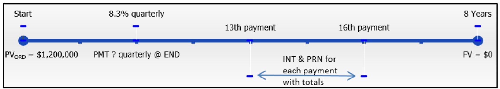
Molson Coors Brewing Company just acquired $1.2 million worth of new brewing equipment for its Canadian operations. The terms of the loan require end-of-quarter payments for eight years at 8.3% compounded quarterly. For accounting purposes, the company is interested in knowing the principal and interest portions of each payment for the fourth year and also wants to know the total interest and principal paid during the year. Construct the partial amortization schedule.
Solution
Construct a partial amortization schedule for the fourth year of the loan along with the total interest and principal paid during the year.
What You Already Know
Step 1:
The timeline for the equipment loan appears in the timeline.
\(PV_{ORD}\) = $1,200,000, \(IY\) = 8.3%, \(CY\) = 4, \(PY\) = 4, Years = 8, \(FV\) = $0
How You Will Get There
Step 1 (continued):
Solve for the payment (\(PMT\)) using Formulas 9.1, 11.1, and 11.4.
Step 2:
Set up the partial amortization table for the ordinary annuity.
Step 3:
Calculate the future value of loan principal for the end of the third year (the 12th payment) using Formulas 9.2 and 9.3. Then calculate the future value of the first 12 payments using Formulas 11.1 and 11.2. Calculate the principal balance after 12 payments through \(BAL = FV − FV_{ORD}\).
Step 4:
Fill in the payment column for the four payments made in the fourth year.
Steps 5 to 8:
For each line of the table, use Formula 13.1 and Formula 13.2 and the rearranged Formula 13.3.
Steps 9 to 11:
Not needed, since the final payment is not involved.
Step 12:
Check for the "missing penny."
Step 13:
Sum the interest and principal portions.
Perform
Step 1 (continued):
\(i=8.3 \% / 4=2.075 \% ; N=4 \times 8=32 \) payments
\[\$ 1,200,000=PMT\left[\dfrac{1-\left[\frac{1}{(1+0.02075)^{\frac{4}{4}}}\right]^{32}}{(1+0.02075)^{\frac{4}{4}}-1}\right] \nonumber \]
\[PMT=\dfrac{\$ 1,200,000}{\left[\frac{0.481701}{0.02075}\right]}=\$ 51,691.71 \nonumber \]
Steps 2 to 11 (with some calculations, including Step 3) are detailed in the table below:
| Payment Number | Payment Amount ($) (PMT) | Interest Portion ($) (INT) | Principal Portion ($) (PRN) | Principal Balance Remaining ($) (PRN) |
|---|---|---|---|---|
| 12 | (1) $ 839,147.91 | |||
| 13 | $51,691.71 | (2) $17,412.32 | (3) $34,279.39 | (4) $804,868.52 |
| 14 | $51,691.71 | $16,701.02 | $34,990.69 | $769,877.83 |
| 15 | $51,691.71 | $15,974.96 | $35,716.75 | $734,161.08 |
| 16 | $51,691.71 | $15,233.84 | $36,457.87 | $697,703.22 |
| Total |
(1) Step 3:
Principal: \(N=4 \times 3=12\) compounds; \(FV=\$ 1,200,000(1+0.02075)^{12}=\$ 1,535,373.036\)
Payments: \(N=4 \times 3=12\) payments;
\(FV_{ORD}=\$ 51,691.71\left[\dfrac{\left[(1+0.02075)^{\frac{4}{4}}\right]^{12}-1}{(1+0.02075)^{\frac{4}{4}}-1}\right]=\$ 51,691.71\left[\dfrac{0.279477}{0.02075}\right]=\$ 696,225.1283 \)
Balance: \( \$ 1,535,373.036-\$ 696,225.1283=\$ 839,147.9072\)
(2) \(INT =\$ 839,147.9072 \times\left((1+0.02075)^{\frac{4}{4}}-1\right)=\$ 17,412.31908\)
(3) \(PRN=\$ 51,691.71-\$ 17,412.31908=\$ 34,279.39092 \)
(4) \(BAL_{P2}=\$ 839,147.9072-\$ 34,279.39092=\$ 804,868.5163\)
Steps 12 to 13:
Adjust for the "missing pennies" (noted in red) and total the interest.
| Payment Number | Payment Amount ($) (PMT) | Interest Portion ($) (INT) | Principal Portion ($) (PRN) | Principal Balance Remaining ($) (PRN) |
|---|---|---|---|---|
| 12 | (1) $ 839,147.91 | |||
| 13 | $51,691.71 | (2) $17,412.32 | (3) $34,279.39 | (4) $804,868.52 |
| 14 | $51,691.71 | $16,701.02 | $34,990.69 | $769,877.83 |
| 15 | $51,691.71 | $15,974.96 | $35,716.75 | $734,161.08 |
| 16 | $51,691.71 | $15,233.85 | $36,457.86 | $697,703.22 |
| Total | $206,766.84 | $65,322.15 | $141,444.69 |
Calculator Instructions
| N | I/Y | PV | PMT | FV | P/Y | C/Y |
|---|---|---|---|---|---|---|
| 32 | 8.3 | 1200000 |
Answer: -51,691.71391 Re-keyed as: -51691.71 |
0 | 4 | 4 |
| Payment | P1 | P2 | BAL (output) | PRN (output) | INT (output) |
|---|---|---|---|---|---|
| 12 | 12 | 12 | 839,147.9072 | N/A | N/A |
| 13 | 13 | 13 | 804,868.5163 | 34,279.39092 | 17,412.31908 |
| 14 | 14 | 14 | 769,877.828 | 34,990.68829 | 16,701.02171 |
| 15 | 15 | 15 | 734,161.083 | 35,716.74507 | 15,974.96493 |
| 16 | 16 | 16 | 697,703.2154 | 36,457.86753 | 15,233.84247 |
| Total | 13 | 16 | 697,703.2154 | 141,444.6918 | 65,322.14819 |
The partial amortization schedule for the fourth year is shown in the table above. The total interest paid in the year is $65,322.15, and the principal portion is $141,444.69