
13.2: Calculating the Final Payment


- Last updated
- Jul 18, 2022
- Save as PDF

( \newcommand{\kernel}{\mathrm{null}\,}\)
If you have ever paid off a loan you may have noticed that your last payment was a slightly different amount than your other payments. Whether you are making monthly insurance premium payments, paying municipal property tax installments, financing your vehicle, paying your mortgage, receiving monies from an investment annuity, or dealing with any other situation where an annuity is extinguished through equal payments, the last payment typically differs from the rest, by as little as one penny or up to a few dollars. This difference can be much larger if you arbitrarily chose an annuity payment as opposed to determining an accurate payment through time value of money calculations.
Why is it important for this final payment to differ from all of the previous payments? From a consumer perspective, you do not want to pay a cent more toward a debt than you have to. In 2011, the average Canadian is more than $100,000 in debt across various financial tools such as car loans, consumer debt, and mortgages. Imagine if you overpaid every one of those debts by a dollar. Over the course of your lifetime those overpayments would add up to hundreds or even thousands of dollars.
On the business side, particularly where companies are collecting debts from customers, two main issues are legality and profitability:
- Legality. A business can legally collect only the exact amount of money its consumers owe and not a penny more. If a business collects more money than it is owed, it is legally obliged to reimburse the consumer or it will face legal repercussions.
- Profitability. RBC has over $200 billion in outstanding loans. What if it told every customer who borrowed money last year that they did not have to worry about paying off that final nickel on their loan? This decision would forego millions in revenue. Shareholders would be very unhappy. Giving up even the tiniest amounts of revenue can aggregate into meaningful losses.
Section 11.5 discussed an approximation technique for the final annuity. It is now time to be precise in this calculation. In the current section, you will see why the final payment differs and how to calculate its exact amount. You will also calculate the principal and interest components for a series of payments involving the final payment.
Why Is the Final Payment Different?
Section 11.4 introduced the calculations to determine the annuity payment. Observe that you always needed to round a non-terminating annuity payment to two decimals. It is rare for a calculated annuity payment not to require rounding. The rounding up or down of the annuity payment forms the basis for adjusting the final payment. Observe the implication of each rounding procedure as summarized in this table.
| How the Payment Was Rounded | Principal Implications | Interest Implications | Final Payment Implications |
|---|---|---|---|
| Upward | Overpayment | Slight decrease | Needs to be reduced in an amount equal to the overpayment and savings on the interest. |
| Downward | Underpayment | Slight increase | Needs to be increased in an amount equal to the underpayment and extra charges on the interest. |
- Annuity Payment Rounded Up. If the calculated annuity payment is exactly
- Annuity Payment Rounded Down. The same principles apply when the annuity payment is rounded down. If you calculated
For example, take a $200,000 loan for 25 years at 6% compounded semi-annually with monthly payments. The calculated
How It Works
The following six steps are needed to calculate the final payment. These steps are designed to integrate with the next section, where the principal and interest components on a series of payments involving the final payment are calculated.
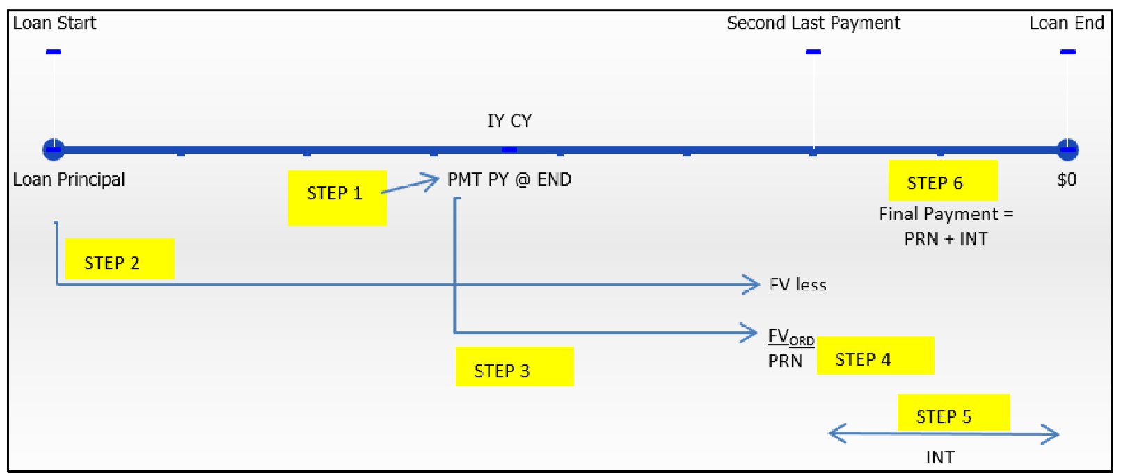
Step 1: Draw a timeline to represent the annuity. A typical timeline format appears in the figure above. Identify all seven time value of money variables. If all are known, proceed to step 2. Most commonly,
Step 2: Calculate the future value of the original principal at
Step 3: To calculate the future value of all annuity payments (
Step 4: Subtract the future value of the payments from the future value of the original principal (step 2 − step 3) to arrive at the principal balance remaining immediately prior to the last payment. This is the principal owing on the account and therefore is the principal portion (
Step 5: Calculate the interest portion (
Step 6: Add the principal portion from step 4 to the interest portion from step 5. The sum is the amount of the final payment.
Important Notes
The calculator determines the final payment amount using the AMORT function described in Section 13.1. To calculate the final payment:
- You must accurately enter all seven time value of money variables (
- Press 2nd AMORT.
- Enter the payment number for the final payment into P1 and press Enter followed by ↓.
- Enter the same payment number for P2 and press Enter followed by ↓.
- In the BAL window, note the balance remaining in the account after the last payment is made. Watch the cash flow sign to properly interpret what to do with it! The sign matches the sign of your PV. The next table summarizes how to handle this balance.
| Type of Transaction | Positive BAL | Negative BAL |
|---|---|---|
| Loan | Increase final payment | Decrease final payment |
| Investment Annuity | Decrease final payment | Increase final payment |
- Loans. For a loan for which
- Investment Annuities. For an investment annuity where
- A helpful key sequence shortcut to arrive at the final payment is to have
- This sequence automatically adjusts the payment accordingly for both loans and investment annuities. Manually round the answer to two decimals when the calculation is complete.
- If you are interested in the
Things To Watch Out For
In Section 11.5 you calculated the
You do not achieve the same answer through the approximation technique, because
Paths To Success
An alternative method to adjust the final payment is to calculate the future value of the rounding error on the payment. Recall the $200,000 loan for 25 years at 6% compounded semi-annually with monthly payments. The calculated
The underpayment is $2.23, which then means the final payment is increased to $1,279.61 + $2.23 = $1,281.84. Note the one disadvantage of this technique is that you are unable to determine the interest and principal components of that final payment. Calculating these components requires you to apply the six-step procedure discussed above.
Consider the following five statements and then answer the two questions that follow.
- The final payment is exactly the same as any other annuity payment.
- The final payment is smaller, reflecting an overpayment of principal of $0.04 plus any lower interest charges saved.
- The final payment is smaller, reflecting an underpayment of principal of $0.04 plus any higher interest charges earned.
- The final payment is larger, reflecting an overpayment of principal of $0.04 plus any lower interest charges saved.
- The final payment is larger, reflecting an underpayment of principal of $0.04 plus any higher interest charges earned.
- If the annuity payment is rounded up by $0.004 per payment and involves 10 payments, which statement is correct?
- If the annuity payment is rounded down by $0.004 per payment and involves 10 payments, which statement is correct?
- Answer
-
- b. When rounding up, principal is reduced faster (overpayment) and more interest is saved.
- e. When rounding down, principal is reduced more slowly (underpayment) and more interest is earned
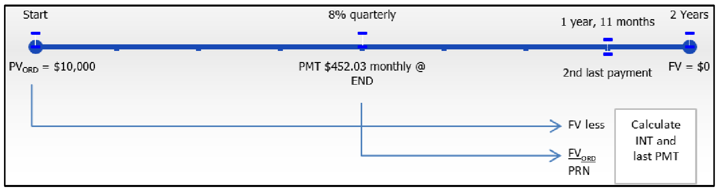
Recall Example 13.1.1, in which Nichols and Burnt borrowed $10,000 at 8% compounded quarterly with month-end payments of $452.03 for two years. The accountant now needs to record the final payment on the loan with correct portions assigned to principal and interest.
Solution
Calculate the principal portion (
What You Already Know
Step 1:
The following information about the accounting firm's loan is known, as illustrated in the timeline.
How You Will Get There
Step 2:
Calculate the future value of the loan principal at the time of the 23rd payment using Formulas 9.1, 9.2, and 9.3.
Step 3:
Calculate the future value of the first 23 payments using Formulas 11.1 and 11.2.
Step 4:
Calculate the principal balance remaining after 23 payments through
Step 5:
Calculate the interest portion by using Formula 13.1.
Step 6:
Calculate the final payment by totaling steps 4 and 5 above.
Perform
Step 2:
Step 3:
Step 4:
Step 5:
Step 6:
Final
Calculator Instructions
| N | I/Y | PV | PMT | FV | P/Y | C/Y |
|---|---|---|---|---|---|---|
| 24 | 8 | 10000 | -452.03 | 0 | 12 | 4 |
| P1 | P2 | BAL (output) | PRN (output) | INT (output) |
|---|---|---|---|---|
| 24 | 24 |
0.061582 *added to payment of $452.03=$452.09 |
449.055627 *added BAL=$449.12 |
2.974372 |
The accountant for Nichols and Burnt should record a final payment of $452.09, which consists of a principal portion of $449.12 and an interest portion of $2.97.
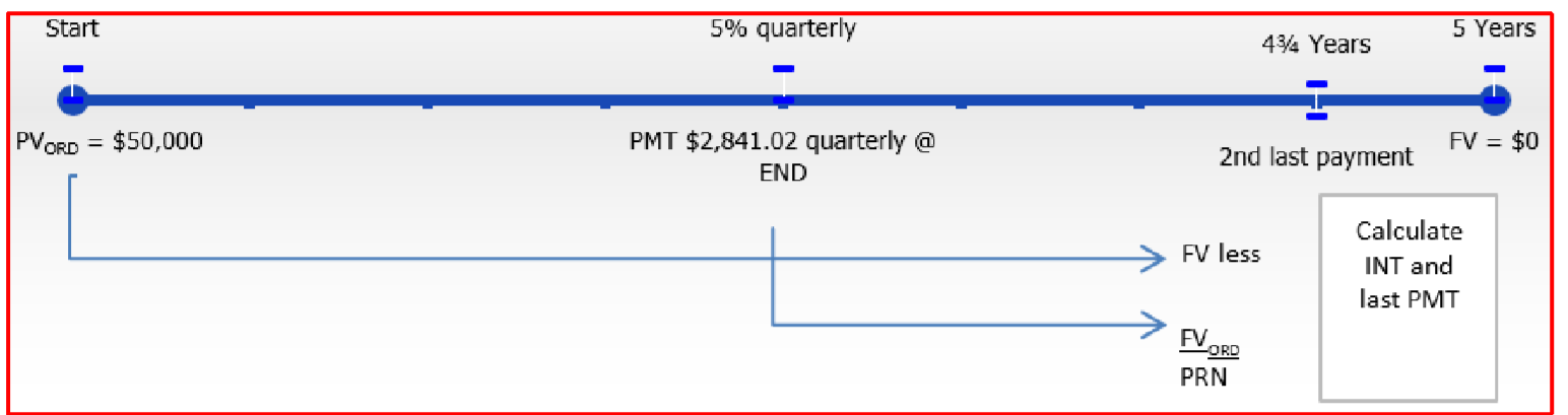
Recall Example 13.1.2, in which Baxter has $50,000 invested into a five-year annuity that earns 5% compounded quarterly and makes regular end-of-quarter payments of $2,841.02 to him. He needs to know the amount of his final payment, along with the principal and interest components.
Solution
Calculate the principal portion (
What You Already Know
Step 1:
You know the following about the investment annuity, as illustrated in the timeline.
How You Will Get There
Step 2:
Calculate the future value of the investment at the time of the 19th payment using Formulas 9.1, 9.2, and 9.3.
Step 3:
Calculate the future value of the first 19 payments using Formulas 11.1 and 11.2.
Step 4:
Calculate the principal balance remaining after 19 payments through
Step 5:
Calculate the interest portion by using Formula 13.1.
Step 6:
Calculate the final payment by totaling steps 4 and 5 above.
Step 2:
Step 3:
Step 4:
Step 5:
Step 6:
Final
Calculator Instructions
| N | I/Y | PV | PMT | FV | P/Y | C/Y |
|---|---|---|---|---|---|---|
| 20 | 5 | -50000 | 2841.02 | 0 | 4 | 4 |
| P1 | P2 | BAL (output) | PRN (output) | INT (output) |
|---|---|---|---|---|
| 20 | 20 |
0.011696 *subtracted from payment of $2,841.02=$2841.01 |
2,805.945823 *subtract BAL=$2,805.93 |
35.074176 |
Baxter will receive a final payment of $2,841.01 consisting of $2,805.93 in principal plus $35.08 in interest.
Calculating Principal and Interest Portions for a Series Involving the Final Payment
Now that you know how to calculate the last payment along with its interest and principal components, it is time to extend this knowledge to calculating the principal and interest portions for a series of payments that involve the final payment.
How It Works
For a series of payments, you follow essentially the same steps as in Section 13.1; however, you need a few minor modifications and interpretations:
Step 1: Draw a timeline. Identify the known time value of money variables, including
Step 2: If the annuity payment amount is known, proceed to step 3. If it is unknown, then solve for the annuity payment using Formulas 9.1 (Periodic Interest Rate) and 11.1 (Number of Annuity Payments) and by rearranging Formula 11.4 (Ordinary Annuity Present Value). Round this payment to two decimals.
Step 3: Calculate the future value of the original principal immediately prior to the series of payments being made. Use Formulas 9.1 (Periodic Interest Rate), 9.2 (Number of Compounding Periods for a Single Payment), and 9.3 (Compound Interest for Single Payments).
Step 4: Calculate the future value of all annuity payments already made prior to the first payment in the series. Apply Formulas 11.1 (Number of Annuity Payments) and 11.2 (Ordinary Annuity Future Value).
Step 5: Calculate the balance (
Step 6: Calculate the future value of the original principal immediately at the end of the timeline. Use Formulas 9.1 (Periodic Interest Rate), 9.2 (Number of Compounding Periods for Single Payments), and 9.3 (Compound Interest for Single Payments).
Step 7: Calculate the future value of all annuity payments, including the unadjusted final payment. Apply Formulas 11.1 (Number of Annuity Payments) and 11.2 (Ordinary Annuity Future Value).
Step 8: Calculate the balance (
Step 9: Calculate the interest portion using Formula 13.4, but modify the final amount by the result from step 8. Hence, Formula 13.4 looks like
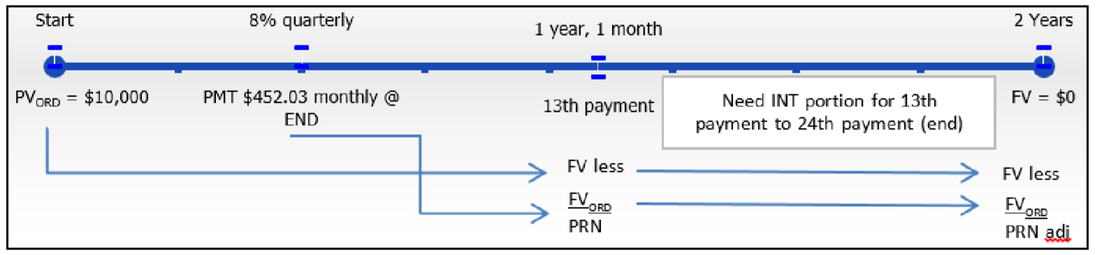
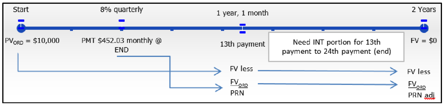
Revisit Example 13.1.1. The accountant at the accounting firm of Nichols and Burnt is completing the tax returns for the company and needs to know the total principal portion and interest expense paid during the tax year encompassing payments 13 through 24 inclusively. Recall that the company borrowed $10,000 at 8% compounded quarterly, with month-end payments of $452.03 for two years.
Solution
Calculate the total principal portion (
What You Already Know
Step 1:
The following information about the accounting firm's loan is known, as illustrated in the timeline.
How You Will Get There
Step 2:
Skip this step, since
Step 3:
Calculate the future value of the loan principal after the 12th payment using Formulas 9.1, 9.2, and 9.3.
Step 4:
Calculate the future value of the first 12 payments using Formulas 11.1 and 11.2.
Step 5:
Calculate the balance remaining after 12 payments through
Step 6:
Calculate the future value of the loan principal after the 24th payment using Formulas 9.2, and 9.3.
Step 7:
Calculate the future value of all 24 payments using Formulas 11.1 and 11.2.
Step 8:
Calculate the balance on the loan after all payments through
Step 9:
Calculate the interest portion by using the adjusted Formula 13.4.
Perform
Step 3:
Step 4:
Step 5:
Step 6:
Step 7:
Step 8:
Step 9:
Calculator Instructions
| N | I/Y | PV | PMT | FV | P/Y | C/Y |
|---|---|---|---|---|---|---|
| 24 | 8 | 10000 | -452.03 | 0 | 12 | 4 |
| P1 | P2 | BAL (output) | PRN (output) | INT (output) |
|---|---|---|---|---|
| 13 | 24 | 0.0615825 |
5,197.890788 *add BAL=$5,197.90 |
226.469212 |
For the tax year covering payments 13 through 24, total payments of $5,424.42 are made, of which $5,197.95 goes toward principal while $226.47 is the interest charged.
Paths To Success
Amortization by definition involves the repayment of loans, which are almost always ordinary in nature. What are the implications if you have an investment annuity due, or the rare occurrence of a loan due?
- Step-by-Step Procedures. Whether you are dealing with ordinary annuities or annuities due, all of the processes and procedures remain unchanged.
- Formulas. Make the appropriate substitutions from
- Excel. The annuity type needs to change from 'Ordinary' to 'Due' (in cell C15 of the data entry screen in the template).
- Time Value of Money Button Calculator Settings. When the calculator is loaded with the time value of money variables, ensure that BGN mode has been set and that if the
- AMORT Function on the BAII Plus Calculator. A special adaptation is required but is not introduced at this time. This special adaptation will be discussed in Section 13.3 on amortization schedules due.