15.1: Net Present Value

Last updated
Save as PDF

Page ID: 22159

Jean-Paul Olivier
Red River College of Applied Arts, Science, & Technology

$ \newcommand{\vecs}[1]{\overset { \scriptstyle \rightharpoonup} {\mathbf{#1}} } $ $ \newcommand{\vecd}[1]{\overset{-\!-\!\rightharpoonup}{\vphantom{a}\smash {#1}}} $$\newcommand{\id}{\mathrm{id}}$ $ \newcommand{\Span}{\mathrm{span}}$ $ \newcommand{\kernel}{\mathrm{null}\,}$ $ \newcommand{\range}{\mathrm{range}\,}$ $ \newcommand{\RealPart}{\mathrm{Re}}$ $ \newcommand{\ImaginaryPart}{\mathrm{Im}}$ $ \newcommand{\Argument}{\mathrm{Arg}}$ $ \newcommand{\norm}[1]{\| #1 \|}$ $ \newcommand{\inner}[2]{\langle #1, #2 \rangle}$ $ \newcommand{\Span}{\mathrm{span}}$ $\newcommand{\id}{\mathrm{id}}$ $ \newcommand{\Span}{\mathrm{span}}$ $ \newcommand{\kernel}{\mathrm{null}\,}$ $ \newcommand{\range}{\mathrm{range}\,}$ $ \newcommand{\RealPart}{\mathrm{Re}}$ $ \newcommand{\ImaginaryPart}{\mathrm{Im}}$ $ \newcommand{\Argument}{\mathrm{Arg}}$ $ \newcommand{\norm}[1]{\| #1 \|}$ $ \newcommand{\inner}[2]{\langle #1, #2 \rangle}$ $ \newcommand{\Span}{\mathrm{span}}$$\newcommand{\AA}{\unicode[.8,0]{x212B}}$

If you decide to pursue a course of action, what is the net benefit or cost of making that decision? How can you tell systematically which choice is financially superior?

Let’s say that your marketing department thinks it has stumbled onto the next hot product to hit the market. The estimated research and development costs are $10 million today with an expected $5 million revitalization cost in five years. The product hits shelves in two years. Estimated year-end profits are $4 million in the first three years and $3 million for the subsequent two years. At that time, the rapid pace of technology will end the life cycle of the new product. This last year will earn an estimated $1 million in profits. The funds needed for this project will be obtained at 12% compounded annually. Does this project make financial sense? Your co-worker argues that the decision is clear: You would spend $15 million to earn $19 million, so the project should go forward. What do you think?

Your co-worker’s analysis summed the nominal numbers. This clearly violates the fundamental concept of time value of money. In this section, we will explore different types of investment decisions and study techniques for making optimal financial decisions.

What Is Involved in Making Monetary Business Decisions?

Investment decisions must consider both the type of decision being made along with the source of funding, which influences the interest rate used in financial calculations.

What Type of Decision Is Being Made?

While there is no such thing as a “standard” or “normal” decision, many business decisions seem to fall into the same three categories:

Decision #1: Making One Choice from Multiple Options. When you face a variety of options that will solve your problem, which option is financially the best?
Decision #2: Deciding Whether to Pursue One Course of Action. When you face only one particular course of action, do you do it or not?
Decision #3: Making Multiple Choices under Constraints. If you have limited resources and many different opportunities from which you can choose more than one, how do you select which opportunities to pursue and which to let pass by?

What Monetary Source Is Being Used and What Does It Cost?

The structure of many decisions follows the old adage that you have to spend money to make money. Many courses of action require an investment up front (costs) to receive the reward (profits) in the future. This means you need to tap a source of money before you can go forward with any course of action. Individuals and corporations can access many of the same monetary sources, but businesses have additional options that are not available to individuals.

Personal Funding Sources. You have limited options for obtaining money. Typically, you can either use debt financing such as a loan from a bank or a line of credit, or you can withdraw money from an investment fund or savings account.
1. If you borrow, the financial cost of the project is the interest rate that is being charged on the borrowed funds. Therefore, if you fund the project using a loan at 8.5% compounded annually, the loan's interest rate becomes the nominal rate you should use in the required time value of money calculations.
2. If you withdraw money from an investment, the cost of this project is the interest rate you forego on those funds. For example, if you take the money out of a GIC earning 4% compounded annually, you should use the GIC's interest rate in the decision calculations.
Business Funding Sources. Businesses have substantially more choices than individuals when obtaining financing. In addition to debt financing and current investments, businesses also can issue bonds or use equity financing, such as offering company shares. Bartering with business partners is also possible. The same principle applies, though: Whatever interest rate the funding source involves carries forward into any decision-making calculations.

The fundamental concept of time value of money states that all money must be moved to the same date before you can compare alternatives fairly. As mentioned above, the source of funding you use determines the interest rate in these calculations. If you use multiple sources to gather the needed funds, your interest rate is a weighted average of all the debt and equity financing rates, and of course if you use a single source then the weighted average is simply the one source’s rate. The weighted interest rate is known as the cost of capital. This textbook assumes the cost of capital in calculations is compounded annually unless otherwise specified.

How to Make the Decision

Businesses most commonly make decisions by performing one of two methods: net present value or internal rates of return. Net present value methods are based on all of the cash flows of a decision expressed in today's dollars. This is the focus of this section. Internal rates of return methods are based on the percentage gains of an investment or the yield of the project, which is discussed in the next section.

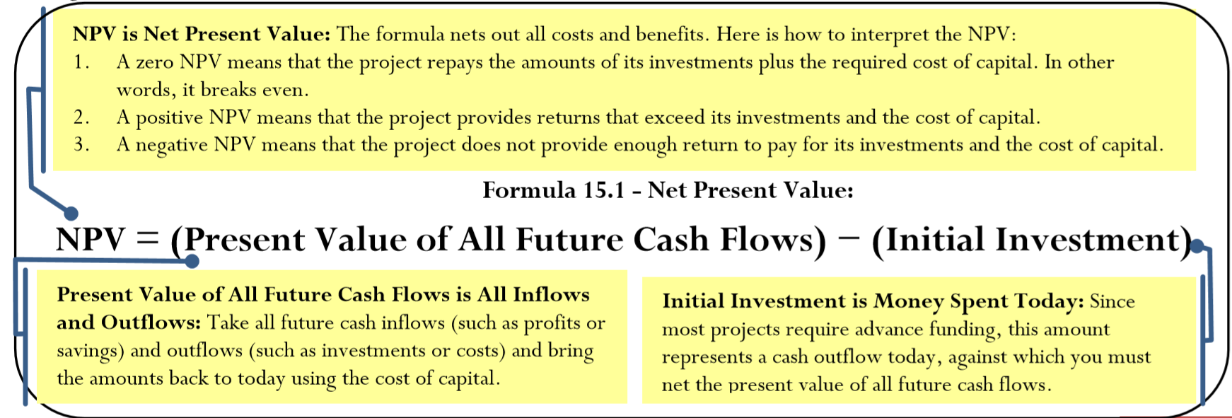
The net present value ($NPV$) method calculates the difference between all benefits and costs for any given project in today's dollars. This decision-making technique calculates the value of all future income and expense streams brought back to today (which serves as the focal date). The word net means that the technique considers the invested money, all costs or expenses, along with all rewards such as profits in its calculations. Remember these criteria for making smart $NPV$ financial decisions:

If the net present value is greater than or equal to $0, the project makes financial sense since it will add value to the company or at minimum break even. It is financially logical to pursue these types of projects.
If the net present value is less than $0, the project does not make financial sense since it will lose money for the company. A company has no financial reason to pursue these types of projects.

Of course, businesses often have many non-financial reasons for pursuing or not pursuing certain courses of action. These reasons are beyond the scope of this textbook.

Observe how $NPV$ relates to each of the three common types of business decision categories:

Decision #1: Making One Choice from Multiple Options. You should choose the project with the best $NPV$. In this section you will learn a technique that helps you choose between projects of identical length. Section 15.2 introduces another technique for choosing between projects of differing length. For example, you cannot simply use $NPV$ to compare project #1, which has a four-year life, against project #2, which has a six-year life.
Decision #2: Choosing Whether to Pursue One Course of Action. You should pursue the project if the $NPV$ is positive or at a minimum zero.
Decision #3: Making Multiple Choices under Constraints. You should choose the projects that maximize the total $NPV$.

This table summarizes the relationship between the three decision types and the financial criteria.

Decision Type	Financial Criteria
Making One Choice from Multiple Options	Best $NPV$
Pursuing One Course of Action	$NPV$ must be $0 or higher
Making Multiple Choices under Constraints	Combination of choices that efficiently maximizes total $NPV$

The Formula

There is no one formula for calculating the net present value. However, you can represent the $NPV$ conceptually through Formula 15.1.

$clipboard_e2a7a66b36a8cc0c93e376aa90d4d3d3c.png$

Formula 15.1

How It Works

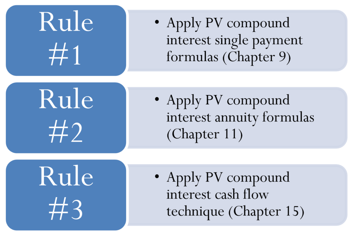
Every decision is different—there is no one definable method to solve a problem. If the solution was obvious, everyone would always make smart decisions! Instead, three rules for moving money will help you choose well:

Rule #1: If there is no regularity to the payments, then each amount represents a single payment. You can calculate the present value of all future cash flows only through the techniques you learned in Chapter 9 for compound interest present value for single payments. Example $\PageIndex{1}$ demonstrates this rule.
Rule #2: If there are regular payments continuously in the same amount, you have an annuity situation. You can calculate the present value of all future cash flows using the techniques from Chapter 11 for compound interest present value for either ordinary annuities or annuities due. Example $\PageIndex{1}$ also demonstrates this rule.
Rule #3: If there are regular payments continuously but in differing amounts, then to use a formula you would have to compute the present value of compound interest single payments as per Rule #1. What distinguishes Rule #3 from Rule #1, though, is the "regularity" characteristic. Under this condition, and assuming that you have access to a financial calculator or spreadsheet, this particular situation presents a shortcut technique called cash flows. Example $\PageIndex{2}$ and Example $\PageIndex{3}$ illustrate these cash flows, which are explained later in this section.

$clipboard_e78459098987079e2f5803c5656bb6d92.png$

Important Notes

When you calculate net present value, most financial forecasts of costs and benefits are best estimates. Therefore, you do not need to be precise to the penny in the final solution. Depending on the dollar amounts involved, companies may commonly round these calculations to the nearest hundred or thousand dollars. While there is no standard practice, this textbook rounds final solutions to the nearest dollar.

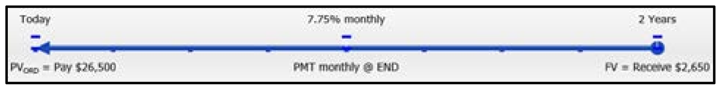
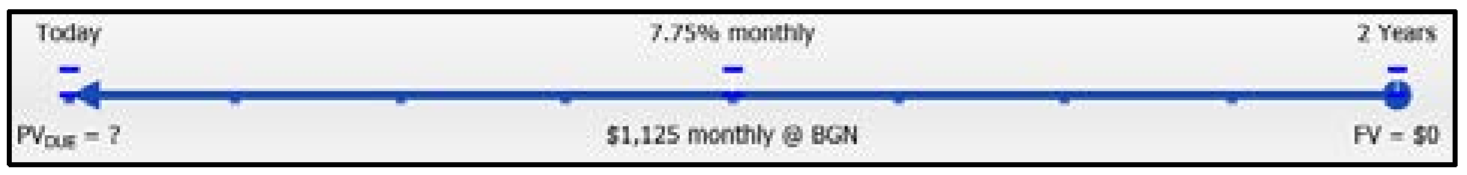
Saggitt Accounting Services needs to regularly update its existing computer workstations. If it leases the workstations for two years, it will make beginning-of-month payments of $1,125 with no residual value. If it purchases the workstations, it will need to pay $26,500 today and it can sell the equipment after two years for 10% of the purchase price. It will need to borrow these funds for two years at 7.75% compounded monthly. Strictly on a financial basis, which option should Saggitt Accounting pursue? How much better is that option in today's dollars?

Solution

Since you need to decide today, you should calculate the net present value ($NPV$) for each alternative. Each of these choices represents a cost, so you choose the option with the lowest $NPV$.

What You Already Know

The timeline for the purchase appears in the first timeline below. With respect to the bank loan itself, present value calculations are not necessary since the present value of all loan payments equals the original loan principal. $PV_{ORD}$ = $26,500, $IY$ = 7.75%, $CY$ = 12, $FV$ = 10% × $26,500 = $2,650, Years = 2 The timeline for the lease appears in the second timeline below. Use the interest rate from the loan in this calculation since Saggitt Accounting would otherwise have to get a loan if it chose not to lease. Therefore, the loan rate represents an appropriate cost of capital. $PMT$ = $1,125, $PY$ = 12, $IY$ = 7.75%, $CY$ = 12, $FV$ = $0, Years = 2

$clipboard_e1638ced54dd28e5ede8b0877ea966cf4.png$

How You Will Get

There Purchase Timeline:

Step 1:

You only need to move the revenue from the end of the second year to today. This is decision Rule #1. Therefore, apply Formulas 9.1, 9.2, and 9.3 rearranging for $PV$.

Step 2:

Calculate $NPV$ using Formula 15.1.

Lease Timeline:

Step 3:

Take the annuity due and move it to today. This is decision Rule #2. Apply Formulas 11.1 and 11.5.

Step 4:

There is no initial investment. Formula 15.1 is then $NPV = PV_{DUE}$.

Step 5:

Calculate the savings by choosing the better option.

$clipboard_ee744eb410bc5dd75187f9bcb4c6ad780.png$

Step 1:

\[i=7.75 \% / 12=0.6458 \overline{3} \% ; N=12 \times 2=24 \text { compounds } \nonumber \]

\[\$ 2,650=PV(1+0.06458 \overline{3})^{24} \nonumber \]

\[PV=\$ 2,650 \div(1+0.06+58 \overline{3})^{24}=\$ 2,270.63 \nonumber \]

Step 2:

\[NPV=\$ 2,270.63-\$ 26,500.00=-\$ 24,229.37 \text { or a cost of } \$ 24,229.37 \nonumber \]

Step 3:

\[N=12 \times 2=24 \text { payments } \nonumber \]

\[PV_{DUE}=\$ 1,125\left[\dfrac{1-\left[\dfrac{1}{\left(1+0.006458 \overline{3}\right)^{\frac{12}{12}}}\right]^{24}}{\left(1+0.006458 \overline{3}\right)^{\frac{12}{12}}}\right] \times\left(1+0.006458 \overline{3}\right)^{\frac{12}{12}}=\$ 25,098.24 \nonumber \]

Step 4:

\[NPV=\text { cost of } \$ 25,098.24 \nonumber \]

Step 5:

\[\$ 25,098.24-\$ 24,229.37=\$ 868.87 \text { savings } \nonumber \]

Calculator instructions:

Transaction	Mode	N	I/Y	PV	PMT	FV	P/Y	C/Y
Purchase	END	24	7.75	Answer:-2,270.631567	0	2650	12	12
Lease	BGN	$\surd$	$\surd$	Answer: -25,098.23508	-1125	0	$\surd$	$\surd$

If Saggitt Accounting Services purchases the machine, it will cost $24,299.37 in today’s dollars. If it leases the machine, it will cost $25,098.24 in today’s dollars. The smart choice is to purchase the machine, realizing a savings of $868.87 in today’s dollars.

A Regular Stream of Cash Flows

A cash flow is a movement of money into or out of a particular project. Therefore, any time you incur a cost or receive a benefit on a particular project, you have a cash flow. Under the three rules for moving money, both single payments and annuities are cash flows. You can move money from a future date to a present date using the existing formulas or calculator techniques.

The third decision rule is for the situation of continuous regular payments that are variable in amount. As indicated in the rule, to solve the problem by formula you would need to calculate compound interest present value (Rule #1) repeatedly. This procedure requires many repetitive calculations in which you calculate $N$ and $PV$ for each cash flow. This is quite cumbersome, since every cash flow introduces two more calculations and another present value to net out. Both the calculator and Excel template simplify this process, reducing both the effort and the chance of error.

As you work with these continuous cash flows, where to put an amount on the timeline depends on whether it is a cost or a benefit.

Costs: Unless otherwise noted, capital costs are spent at the beginning of any time segment. Thus, if there are capital costs in year two, you can assume you incur them at the beginning of year two, which is the same as the end of year one.
Benefits: Revenues, net profits (product sales minus product costs), or other benefits are realized at the end of any time segment. Thus, if there are net profits in year two, you can assume you realize them at the end of year two.

How It Works

Follow these steps when working with regular cash flows of varying amounts:

Step 1: Draw a timeline illustrating all of the cash flows, cost of capital, and any initial investment. Always draw your timeline in an ordinary annuity format with all transactions occurring at the end of each time interval. Thus, any costs you incur at the beginning of a time segment are placed at the end of the prior time segment (unless noted otherwise).

Step 2: For any particular point on the timeline at which more than one cash flow exists, net all cash flows into a single number.

Step 3: Move each cash flow to its present value. If using formulas, calculate the periodic interest rate from Formula 9.1. Follow this calculation by repeatedly applying Formulas 9.2 (Number of Compound Periods for Single Payments) and 9.3 (Compound Interest for Single Payments). Alternatively, if using technology then apply the technique discussed in the appropriate section below.

Step 4: Net the results using Formula 15.1 to arrive at the $NPV$.

Important Notes

Using the BAII Plus Cash Flow Worksheet.

The cash flow function of the calculator requires the cash flows to be regular (such as every month or every quarter or every year). The payment amounts can be the same or variable. If the regularity assumption is not met, do not use the cash flow function; instead solve the problem using Rule #1 for compound interest single payments.

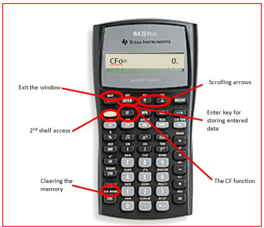
$clipboard_e0ae1455d17e2786764aed314f1f50a50.png$

The photo illustrates the buttons used in the cash flow function of your BAII Plus calculator. Access the cash flow function by pressing CF on the keypad. Immediately clear the memory using 2nd CLR Work to delete any previously entered data. Use the ↑ and ↓ arrows to scroll through the various lines. You must strictly obey the cash flow sign convention and press Enter after keying in any data.

Here are the various lines appearing in the cash flow function:

$CF_o$ = any cash flow today
$CXX$ = a particular cash flow, where $XX$ is the cash flow number starting with 01. You must key in the cash flows in order from the first time segment to the last. You cannot skip a time segment even if it has a value of zero. Each time segment is a placeholder on the timeline.
$FXX$ = the frequency of a particular cash flow, where $XX$ is the cash flow number. It is how many times in a row the corresponding cash flow amount occurs. This allows you to enter recurring amounts instead of keying them in separately. By default, the calculator sets this variable to 1.

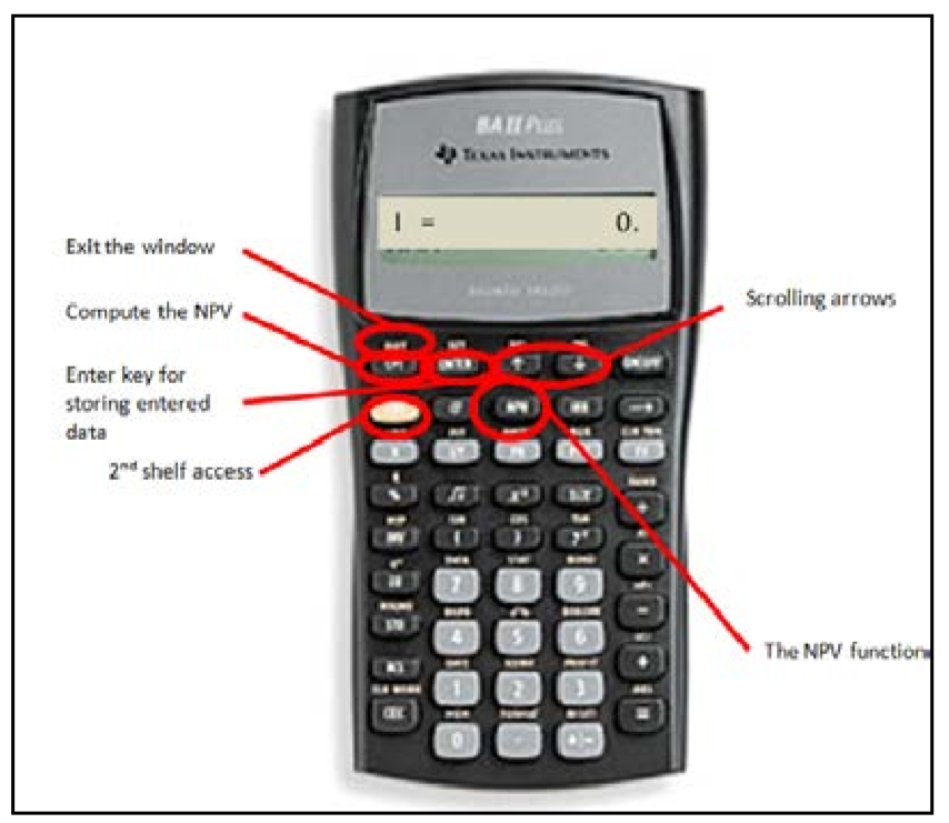
$clipboard_ec15899d409c3e194046b5db6e41cf7c9.png$

Once you have entered all cash flows, you must access other functions to generate the output. For net present value, press $NPV$ on the keypad as illustrated in the photo. This window has two lines:

$I$ = the matching periodic interest rate for the interval of each time segment. If the timeline is drawn with yearly intervals, then this must be the annual cost of capital. If the timeline is drawn with semi-annual intervals, this needs to be the matching semi-annual periodic cost of capital.
$NPV$ = the net present value. Press CPT to calculate this amount. The output nets all future cash flows against any initial investment. This key executes Formula 15.1.

Things To Watch Out For

The most common mistake in using the BAII Plus calculator is failing to enter the matching periodic interest rate in the $NPV$ window. Always check the following:

The compounding on the cost of capital must match the interval between cash flows. If not, convert the rate to match. For example, if your intervals are semi-annual but your cost of capital is annual, you must convert the cost of capital to its equivalent semi-annually compounded rate.
Apply Formula 9.1, being sure to enter the periodic rate and not the nominal rate of interest.

Paths To Success

Since cash flows can be inflows or outflows, it avoids confusion to write all numbers with their cash flow sign conventions onto the timeline. This helps you keep track of the different flows and minimizes the possibility of incorrectly netting out all present values.

Give It Some Thought

If a negative net present value is calculated, does that mean the project is unprofitable?

Answer: No, it means the project cannot recover its investments and the cost of capital. If the company can sufficiently lower its cost of capital, then the net present value may in fact become positive

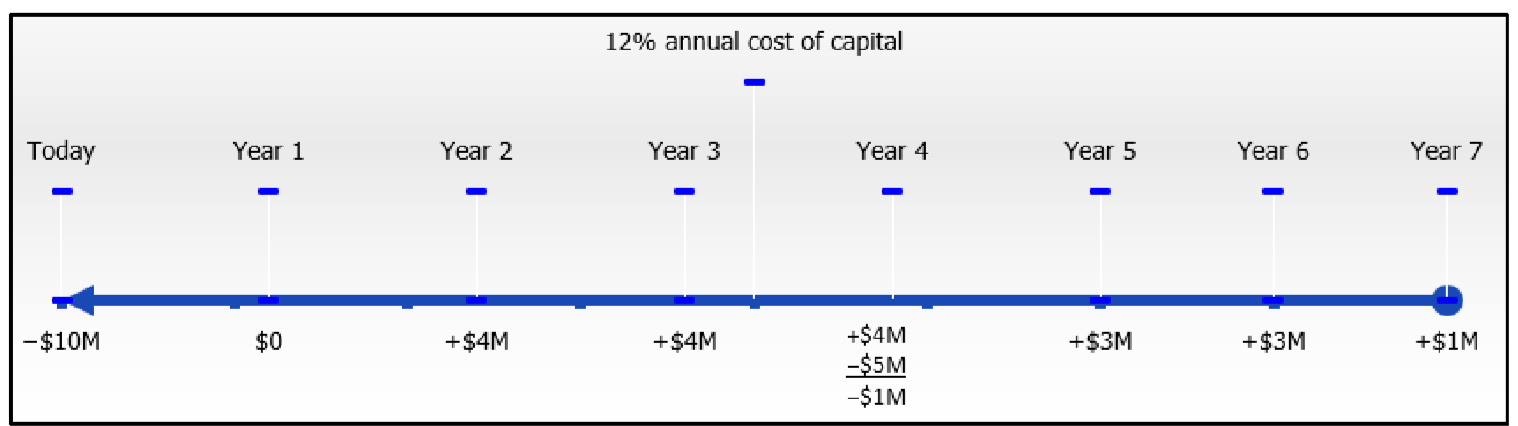
Example $\PageIndex{2}$: Decision #2: Pursuing a Particular Option

Revisit the new product launch discussed in the opening scenario in this section. Recall that research and development costs are $10 million today with an expected revitalization cost of $5 million in the fifth year. The product is expected to go on sale starting in two years and is forecast to produce year-end profits of $4 million for the first three years and another $3 million per year for the subsequent two years. Its last year will earn a projected $1 million in profit. The cost of capital for this project is 12% compounded annually. From a financial perspective only, should this new product be launched?

Solution

You have cash flows on many different dates. In order to decide today, you should move all monies to today and calculate the net present value ($NPV$).

What You Already Know

Steps 1 and 2:

The timeline for the proposed product launch appears below.

\[IY=12 \%, CY=1, PV=-\$ 10 M \nonumber \]

Future cash flows are shown in the timeline. Note that the cost in the fifth year occurs at the beginning of the year, which is the same point in time as the end of the fourth year.

How You Will Get There

Step 3:

Calculate the periodic interest rate by using Formula 9.1. For each cash flow, calculate the present value using Formulas 9.2 and 9.3, rearranging for $PV$.

\[\begin{array}{l}{i=12 \% / 1=12 \%} \\ {\text { Cash Flow } 1: N=1 \times 2=2 \text { compounds; } P V=\$ 4,000,000 \div(1+0.12)^{2}=\$ 3,188,775.51} \\ {\text { Cash Flow } 2: N=1 \times 3=3 \text { compounds; } P V=\$ 4,000,000 \div(1+0.12)^{3}=\$ 2,847,120.991} \\ {\text { Cash Flow } 3: N=1 \times 4=4 \text { compounds; } P V=-\$ 1,000,000 \div(1+0.12)^{5}=\$ 1,702,280.567} \\ {\text { Cash Flow } 4: N=1 \times 5=5 \text { compounds; } P V=\$ 3,000,000 \div(1+0.12)^{6}=\$ 1,519,893.367} \\ {\text { Cash Flow } 6: N=1 \times 7=7 \text { compounds; } P V=\$ 1,000,000 \div(1+0.12)^{7}=\$ 452,349.2153}\end{array} \nonumber \]

Step 4:

Calculate $NPV$ by using Formula 15.1.

\[\begin{aligned} NPV &=(\$ 3,188,775.51+\$ 2,847,120.991-\$ 635,518.0784+\$ 1,702,280.567+\$ 1,519,893.364+ \$ 452,349.2153)-\$ 10,000,000\\&=\$ 9,074,901.569-\$ 10,000,000\\&=-\$ 925,098.43\\ &==>-\$ 925,098 \end{aligned} \nonumber \]

$clipboard_e856443037fd2cf9db78f372625f51974.png$

Perform

Step 3:

$i$ = 12%/1 = 12%

\[\begin{aligned}
&\text { Cash Flow } 1: N=1 \times 2=2 \text { compounds; } PV=\$ 4,000,000 \div(1+0.12)^{2}=\$ 3,188,775.51\\
&\text { Cash Flow } 2: N=1 \times 3=3 \text { compounds; } PV=\$ 4,000,000 \div(1+0.12)^{3}=\$ 2,847,120.991\\
&\text { Cash Flow } 3: N=1 \times 4=4 \text { compounds; } PV=-\$1,000,000 \div(1+0.12)^{4}=-\$ 635,518.0784\\
&\text { Cash Flow } 4: N=1 \times 5=5 \text { compounds; } PV=\$ 3,000,000 \div(1+0.12)^{5}=\$ 1,702,280.567\\
&\text { Cash Flow } 5: N=1 \times 6=6 \text { compounds; } PV=\$ 3,000,000 \div(1+0.12)^{6}=\$ 1,519,893.364\\
&\text { Cash Flow } 6: N=1 \times 7=7 \text { compounds; } PV=\$ 1,000,000 \div(1+0.12)^{7}=\$ 452,349.2153
\end{aligned} \nonumber \]

Step 4:

\[\begin{aligned} NPV &= (\$3,188,775.51 + \$2,847,120.991 − \$635,518.0784 + \$1,702,280.567 + \$1,519,893.364 + \$452,349.2153) − \$10,000,000 \\ &= \$9,074,901.569 − \$10,000,000\\ &= −\$925,098.43 \\ &==> −\$925,098 \end{aligned} \nonumber \]

Calculator Instructions

Cash Flows
Cash Flow	Amount ($CXX$	Frequency ($FXX$)
CFO	-10000000	N/A
C01 & F01	0	1
C02 & F02	4000000	2
C03 & F03	-1000000	1
C04 & F04	3000000	2
C05 & F05	1000000	1

NPV
I	NPV
12	Answer: -925,098.4309

If the forecasted costs and profits are reasonably accurate, then the new product should not be launched under the current financial structure since its net present value is −$925,098. This means that the profits are unable to recover the investments required along with the cost of capital.

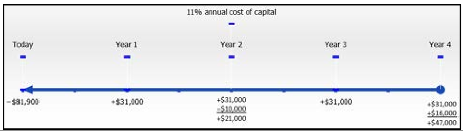
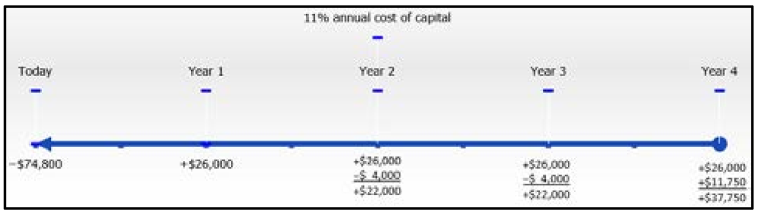
Example $\PageIndex{3}$: Decision #1: Choosing between Options with Cash Flows

Lethbridge Community College is considering purchasing new industrial photocopier equipment and has narrowed the choices down to two comparable Xerox and Canon machines. The Xerox machine can be acquired for $81,900 today and is expected to have a life of four years with savings of $31,000 in labour and materials each year. A $10,000 maintenance package is expected to be purchased at the beginning of year three, and the machine can be sold for $16,000 after the four years. The Canon machine retails for $74,800 and is forecasted to save $26,000 in labour and materials each year. A $4,000 maintenance procedure is needed at the beginning of both years three and four. The salvage value of the machine is estimated at $11,750. The cost of capital is 11%. Which machine should be purchased, and how much money will it save over the alternative?

Solution

For each photocopier, you have cash flows on many different dates. In order to decide today, you should move all monies to today and calculate the net present value ($NPV$) for each photocopier.

What You Already Know

Steps 1 and 2:

The timelines for each photocopier appear below (Xerox on left, Canon on right).

Xerox: $IY=11 \%, CY=1, PV=-\$ 81,900$, future cash flows are shown in the timeline.

Canon: $IY=11 \%, CY=1, PV=-\$ 74,800$, future cash flows are shown in the timeline.

Note that costs occurring at the beginning of the year are recorded at the end of the previous year.

$clipboard_e3110f06e936818bf2762a9e2e8eef060.png$

How You Will Get There

Step 3:

Calculate the periodic interest rate by using Formula 9.1.For each photocopier, calculate the present value of each cash flow using Formulas 9.2 and 9.3, rearranging for $PV$.

Step 4:

For each photocopier, calculate $NPV$ by using Formula 15.1.

Step 5:

Calculate the savings by choosing the better option.

$clipboard_e6fe386b54bfbdb9e1bb312a788609090.png$

Perform

Step 3:

\[i=11 \% / 1=11 \% \nonumber \]

Xerox:

\[\begin{array}{l}{\text { Cash Flow } 1: N=1 \times 1=1 \text { compounds; } PV=\$ 31,000 \div(1+0.11)^{1}=\$ 27,927.\overline{927}} \\ {\text { Cash Flow } 2: N=1 \times 2=2 \text { compounds; } PV=\$ 21,000 \div(1+0.11)^{2}=\$ 17,044.0711} \\ {\text { Cash Flow } 3: N=1 \times 3=3 \text { compounds; } PV=\$ 31,000 \div(1+0.11)^{3}=\$ 22,666.93282} \\ {\text { Cash Flow } 4: N=1 \times 4=4 \text { compounds; } PV=\$ 47,000 \div(1+0.11)^{4}=\$ 30,960.35578}\end{array} \nonumber \]

Step 4:

\[\begin{aligned} NPV &=(\$ 27,927.\overline{927}+\$ 17,044.0711+\$ 22,666.93282+\$ 30,960.35578)-\$ 81,900 \\ &=\$ 98,599.28763-\$ 81,900\\ &=\$ 16,699.29\\ &==>\$ 16,699 \end{aligned} \nonumber \]

Canon:

\[\begin{array}{l}{\text { Cash Flow } 1: N=1 \times 1=1 \text { compounds; } PV=\$ 26,000 \div(1+0.11)^{1}=\$ 23,423 . \overline{423}} \\ {\text { Cash Flow } 2: N=1 \times 2=2 \text { compounds; } PV=\$ 22,000 \div(1+0.11)^{2}=\$ 17,855.69353} \\ {\text { Cash Flow } 3: N=1 \times 3=3 \text { compounds; } PV=\$ 22,000 \div(1+0.11)^{3}=\$ 16,086.21039} \\ {\text { Cash Flow } 4: N=1 \times 4=4 \text { compounds; } PV=\$ 37,750 \div(1+0.11)^{4}=\$ 24,867.09427}\end{array} \nonumber \]

Step 4:

Canon:

\[\begin{aligned} NPV &=(\$ 23,423.\overline{423}+\$ 17,855.69353+\$ 16,086.21039+\$ 24,867.09427)-\$ 74,800 \\ &=\$ 82,232.42162-\$ 74,800\\ &=\$ 7,432.42\\ &==>\$ 7,432 \end{aligned} \nonumber \]

Xerox has higher savings by $\$16,699 − \$7,432 = \$9,267$

Step 5:

Xerox has higher savings by $16,699 − $7,432 = $9,267

Calculator Instructions

Cash Flows
	Xerox		Canon
Cash Flow	Amount ($CXX$	Frequency ($FXX$)	Amount ($CXX$	Frequency ($FXX$)
CFO	-81900	N/A	-74800	N/A
C01 & F01	31000	1	26000	1
C02 & F02	21000	1	22000	2
C03 & F03	31000	1	37750	1
C04 & F04	47000	1

NPV
	Xerox	Canon
I	11	11
NPV	Answer: 16,699.28763	Answer: 7,432.421617

Based on the estimated costs, maintenance, and savings, the Xerox photocopier should be purchased because it results in an expected savings of $8,867 in today's dollars. The Xerox machine represents a current cash flow of $16,299, while the Canon is $7,432.

Working with Limited Resources

In an ideal financial world, you should always pursue any project with a positive net present value since that decision results in a financial gain. However, no one, whether an individual person or a large corporation or a government, actually has access to unlimited resources to fund all its potential projects. If such unlimited resources existed, the world's problems could be solved in a day!

There are usually many paths in life that you can choose, each with its own merits. These paths are not necessarily mutually exclusive, so you could choose more than one. However, having limited resources means that you cannot pursue all of these paths. For example, perhaps PepsiCo has learned through market research that it could launch 15 new flavours and types of soft drinks. Each of these flavours and types requires vast production resources, labour demands, and marketing support to bring it to market. But even a company as huge as PepsiCo does not have the resources to pursue all of these opportunities. Which one or ones does it select?

A process called hard capital rationing is used to decide. This process requires you to calculate the net present value of each possible project and then allocate your limited capital resources to the projects efficiently to maximize the combined net present value. From a financial perspective, you do not consider any projects with a negative net present value.

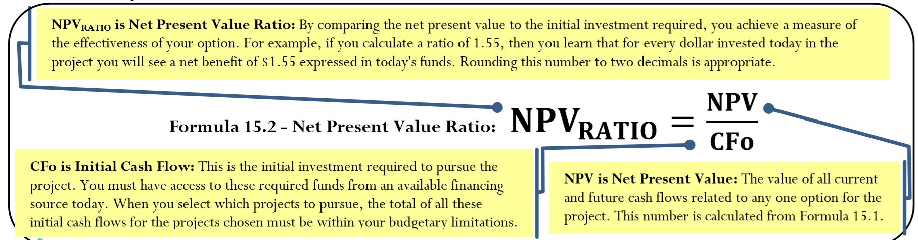
The Formula

The goal in choosing multiple options is to maximize the net present value. In selecting these various options, it is unfair to compare projects of different magnitudes simply by looking at their $NPV$. One would expect that a project requiring a $10 million investment should produce a much larger $NPV$ than a project requiring a $10,000 investment. Instead, it is proper to examine the efficient usage of these limited resources, or to look at the "bang for your buck." This requires you to calculate the net present value ratio shown in Formula 15.2.

$clipboard_e5b2846397cfea7fe2bc0b22405f4379f.png$

Formula 15.2

How It Works

Follow these steps to perform hard capital rationing:

Step 1: Identify the budget constraints.

Step 2: If not already known, calculate the net present value ($NPV$) for each of the available projects using Formula 15.1.

Step 3: Calculate the net present value ratio for each project using Formula 15.2.

Step 4: Rank the projects from the highest to lowest ratios, noting the initial cash flow required under each project.

Step 5: Starting with the project with the highest net present value ratio and progressing through the ranked list of projects, assess different combinations of projects and their total $NPV$ such that the total initial cash flows remain within the budget constraint.

Step 6: Choose the combination that maximizes the $NPV$.

Important Notes

This technique makes the assumption that each of the projects being considered is independent of the others. In other words, choosing one particular project or path does not prevent another project or path from being chosen. There are much more advanced techniques for optimizing a list of projects. These techniques include management sciences or linear programming methods. However, these techniques are beyond the scope of this textbook, which focuses simply on the basic principles behind this decision.

Paths To Success

When completing step 5 of the process, always select the highest $NPV_{RATIO}$ projects in order until you reach a point where the remaining budget becomes an issue. In other words, only at the point where the selection of the next ranked project eliminates a lower-ranked project from consideration do you need to start examining the different possible combinations. In most typical situations, the optimal combination includes all projects selected before this critical point.

Example $\PageIndex{4}$: Decision #3: Working with Limited Resources

Nygard International has identified several projects that it can pursue, as listed in the table below. The current finances of the company permit a capital budget of $1.25 million. Which projects should be undertaken?

Project	Initial Cash Flow	Net Present Value
Automate a production process	$428,000	$214,000
Launch new fashion A	$780,000	$550,000
Replace machinery in distribution centre	$150,000	$175,000
Launch new fashion B	$395,000	$610,000
Expand a retail outlet	$145,000	$245,000
Revise delivery processes	$282,000	$420,000

Solution

You need to perform hard capital rationing to maximize your $NPV$ within your limited budget. This requires you to calculate the net present value ratio ($NPV_{RATIO}$) for each project.

What You Already Know

Step 1:

The total budget available is $1.25 million.

Step 2:

The net present values are provided in the table.

How You Will Get There

Step 3:

Calculate the net present value ratio for each project using Formula 15.2.

Steps 4 to 6:

Rank the $NPV_{RATIO}$ from highest to lowest, assess the budget and combinations available, and then choose the possibility that maximizes $NPV$.

Perform

Steps 3 to 5:

The $NPV_{RATIO}$ is shown in the table below. Projects are sorted into descending order. A few calculations listed below the table show how the $NPV_{RATIO}$ is calculated. Note that after you select the first project, if you were to select the second project then this would eliminate the fifth project since its initial cash flow exceeds the remaining budget ($1,250,000 − $145,000 − $395,000 = $710,000 remaining). Therefore, you always include the first project in your combinations and must explore various arrangements of the next five projects.

Project	Initial Cash Flow	Net Present Value	Net Present Value Ratio	Some Possible Combinations
				1	2	3	4	5
Expand a retail outlet	$145,000	$245,000	(1)1.69	.	.	.	.	.
Launch new fashion B	$395,000	$610,000	(2)1.54	.	.	.
Revise delivery processes	$282,000	$420,000	1.49	.	.		.	.
Replace machinery in distribution centre	$150,000	$175,000	1.17	.		.	.
Launch new fashion A	$780,000	$550,000	0.71					.
Automate a production process	$428,000	$214,000	0.50		.	.	.

(1) $NPV_{RATIO}=\dfrac{\$ 245,000}{\$145,000}=1.69 \nonumber$

(2) $NPV_{RATIO}=\dfrac{\$ 610,000}{\$395,000}=1.54 \nonumber$

	Combinations
	1	2	3	4	5
Total Budget	(1) $972,000	$1,250,000	$1,118,000	$1,005,000	$1,207,000
Total $NPV$	(2) $1,450,000	$1,489,000	$1,244,000	$1,054,000	$1,215,000

(1) $145,000 + $395,000 + $282,000 + $150,000 = $972,000

(2) $245,000 + $610,000 + $420,000 + $175,000 = $1,450,000

Step 6:

Combination #2 offers the highest $NPV$ of $1,489,000.

After the projects are ranked from highest to lowest $NPV$ ratio, the "Expand a retail outlet" offered the highest ratio and is selected. Combination #2, consisting of "Expand a retail outlet," "Launch new fashion B," "Revise delivery processes," and "Automate a production process" offers the highest $NPV$ of $1,489,000 and uses the full $1,250,000 capital budget.

Contributors and Attributions

Template:ContribBusiMathOlivier

Search

Give It Some Thought

Example \(\PageIndex{2}\): Decision #2: Pursuing a Particular Option

Example \(\PageIndex{3}\): Decision #1: Choosing between Options with Cash Flows

Example \(\PageIndex{4}\): Decision #3: Working with Limited Resources

Decision Type	Financial Criteria
Making One Choice from Multiple Options	Best \(NPV\)
Pursuing One Course of Action	\(NPV\) must be $0 or higher
Making Multiple Choices under Constraints	Combination of choices that efficiently maximizes total \(NPV\)

Cash Flows
Cash Flow	Amount (\(CXX\)	Frequency (\(FXX\))
CFO	-10000000	N/A
C01 & F01	0	1
C02 & F02	4000000	2
C03 & F03	-1000000	1
C04 & F04	3000000	2
C05 & F05	1000000	1