
5.2: Diploid Genetics
- Page ID
- 93512

\( \newcommand{\vecs}[1]{\overset { \scriptstyle \rightharpoonup} {\mathbf{#1}} } \)
\( \newcommand{\vecd}[1]{\overset{-\!-\!\rightharpoonup}{\vphantom{a}\smash {#1}}} \)
\( \newcommand{\dsum}{\displaystyle\sum\limits} \)
\( \newcommand{\dint}{\displaystyle\int\limits} \)
\( \newcommand{\dlim}{\displaystyle\lim\limits} \)
\( \newcommand{\id}{\mathrm{id}}\) \( \newcommand{\Span}{\mathrm{span}}\)
( \newcommand{\kernel}{\mathrm{null}\,}\) \( \newcommand{\range}{\mathrm{range}\,}\)
\( \newcommand{\RealPart}{\mathrm{Re}}\) \( \newcommand{\ImaginaryPart}{\mathrm{Im}}\)
\( \newcommand{\Argument}{\mathrm{Arg}}\) \( \newcommand{\norm}[1]{\| #1 \|}\)
\( \newcommand{\inner}[2]{\langle #1, #2 \rangle}\)
\( \newcommand{\Span}{\mathrm{span}}\)
\( \newcommand{\id}{\mathrm{id}}\)
\( \newcommand{\Span}{\mathrm{span}}\)
\( \newcommand{\kernel}{\mathrm{null}\,}\)
\( \newcommand{\range}{\mathrm{range}\,}\)
\( \newcommand{\RealPart}{\mathrm{Re}}\)
\( \newcommand{\ImaginaryPart}{\mathrm{Im}}\)
\( \newcommand{\Argument}{\mathrm{Arg}}\)
\( \newcommand{\norm}[1]{\| #1 \|}\)
\( \newcommand{\inner}[2]{\langle #1, #2 \rangle}\)
\( \newcommand{\Span}{\mathrm{span}}\) \( \newcommand{\AA}{\unicode[.8,0]{x212B}}\)
\( \newcommand{\vectorA}[1]{\vec{#1}} % arrow\)
\( \newcommand{\vectorAt}[1]{\vec{\text{#1}}} % arrow\)
\( \newcommand{\vectorB}[1]{\overset { \scriptstyle \rightharpoonup} {\mathbf{#1}} } \)
\( \newcommand{\vectorC}[1]{\textbf{#1}} \)
\( \newcommand{\vectorD}[1]{\overrightarrow{#1}} \)
\( \newcommand{\vectorDt}[1]{\overrightarrow{\text{#1}}} \)
\( \newcommand{\vectE}[1]{\overset{-\!-\!\rightharpoonup}{\vphantom{a}\smash{\mathbf {#1}}}} \)
\( \newcommand{\vecs}[1]{\overset { \scriptstyle \rightharpoonup} {\mathbf{#1}} } \)
\(\newcommand{\longvect}{\overrightarrow}\)
\( \newcommand{\vecd}[1]{\overset{-\!-\!\rightharpoonup}{\vphantom{a}\smash {#1}}} \)
\(\newcommand{\avec}{\mathbf a}\) \(\newcommand{\bvec}{\mathbf b}\) \(\newcommand{\cvec}{\mathbf c}\) \(\newcommand{\dvec}{\mathbf d}\) \(\newcommand{\dtil}{\widetilde{\mathbf d}}\) \(\newcommand{\evec}{\mathbf e}\) \(\newcommand{\fvec}{\mathbf f}\) \(\newcommand{\nvec}{\mathbf n}\) \(\newcommand{\pvec}{\mathbf p}\) \(\newcommand{\qvec}{\mathbf q}\) \(\newcommand{\svec}{\mathbf s}\) \(\newcommand{\tvec}{\mathbf t}\) \(\newcommand{\uvec}{\mathbf u}\) \(\newcommand{\vvec}{\mathbf v}\) \(\newcommand{\wvec}{\mathbf w}\) \(\newcommand{\xvec}{\mathbf x}\) \(\newcommand{\yvec}{\mathbf y}\) \(\newcommand{\zvec}{\mathbf z}\) \(\newcommand{\rvec}{\mathbf r}\) \(\newcommand{\mvec}{\mathbf m}\) \(\newcommand{\zerovec}{\mathbf 0}\) \(\newcommand{\onevec}{\mathbf 1}\) \(\newcommand{\real}{\mathbb R}\) \(\newcommand{\twovec}[2]{\left[\begin{array}{r}#1 \\ #2 \end{array}\right]}\) \(\newcommand{\ctwovec}[2]{\left[\begin{array}{c}#1 \\ #2 \end{array}\right]}\) \(\newcommand{\threevec}[3]{\left[\begin{array}{r}#1 \\ #2 \\ #3 \end{array}\right]}\) \(\newcommand{\cthreevec}[3]{\left[\begin{array}{c}#1 \\ #2 \\ #3 \end{array}\right]}\) \(\newcommand{\fourvec}[4]{\left[\begin{array}{r}#1 \\ #2 \\ #3 \\ #4 \end{array}\right]}\) \(\newcommand{\cfourvec}[4]{\left[\begin{array}{c}#1 \\ #2 \\ #3 \\ #4 \end{array}\right]}\) \(\newcommand{\fivevec}[5]{\left[\begin{array}{r}#1 \\ #2 \\ #3 \\ #4 \\ #5 \\ \end{array}\right]}\) \(\newcommand{\cfivevec}[5]{\left[\begin{array}{c}#1 \\ #2 \\ #3 \\ #4 \\ #5 \\ \end{array}\right]}\) \(\newcommand{\mattwo}[4]{\left[\begin{array}{rr}#1 \amp #2 \\ #3 \amp #4 \\ \end{array}\right]}\) \(\newcommand{\laspan}[1]{\text{Span}\{#1\}}\) \(\newcommand{\bcal}{\cal B}\) \(\newcommand{\ccal}{\cal C}\) \(\newcommand{\scal}{\cal S}\) \(\newcommand{\wcal}{\cal W}\) \(\newcommand{\ecal}{\cal E}\) \(\newcommand{\coords}[2]{\left\{#1\right\}_{#2}}\) \(\newcommand{\gray}[1]{\color{gray}{#1}}\) \(\newcommand{\lgray}[1]{\color{lightgray}{#1}}\) \(\newcommand{\rank}{\operatorname{rank}}\) \(\newcommand{\row}{\text{Row}}\) \(\newcommand{\col}{\text{Col}}\) \(\renewcommand{\row}{\text{Row}}\) \(\newcommand{\nul}{\text{Nul}}\) \(\newcommand{\var}{\text{Var}}\) \(\newcommand{\corr}{\text{corr}}\) \(\newcommand{\len}[1]{\left|#1\right|}\) \(\newcommand{\bbar}{\overline{\bvec}}\) \(\newcommand{\bhat}{\widehat{\bvec}}\) \(\newcommand{\bperp}{\bvec^\perp}\) \(\newcommand{\xhat}{\widehat{\xvec}}\) \(\newcommand{\vhat}{\widehat{\vvec}}\) \(\newcommand{\uhat}{\widehat{\uvec}}\) \(\newcommand{\what}{\widehat{\wvec}}\) \(\newcommand{\Sighat}{\widehat{\Sigma}}\) \(\newcommand{\lt}{<}\) \(\newcommand{\gt}{>}\) \(\newcommand{\amp}{&}\) \(\definecolor{fillinmathshade}{gray}{0.9}\)Most sexually reproducing species are diploid. In particular, our species Homo sapiens is diploid with two exceptions: we are haploid at the gamete stage (sperm and unfertilized egg); and males are haploid for most genes on the unmatched \(X\) and \(Y\) sex chromosomes (females are \(X X\) and diploid). This latter seemingly innocent fact is of great significance to males suffering from genetic diseases due to an X-linked recessive mutation inherited from their mother. Females inheriting this mutation are most probably disease-free because of the functional gene inherited from their father.
A polymorphic gene with alleles \(A\) and \(a\) can appear in a diploid gene as three distinct genotypes: \(A A, A a\) and \(a a\). Conventionally, we denote \(A\) to be the wildtype allele and \(a\) the mutant allele. Table \(5.4\) presents the terminology of diploidy.
As for haploid genetics, we will determine evolution equations for allele and/or genotype frequencies. To develop the appropriate definitions and relations, we initially assume a population of size \(N\) (which we will later take to be infinite), and assume that the number of individuals with genotypes \(A A, A a\) and \(a a\) are \(N_{A A}\), \(N_{A a}\) and \(N_{a a} .\) Now, \(N=N_{A A}+N_{A a}+N_{a a}\). Define genotype frequencies \(P, Q\) and \(R\) as
\[P=\frac{N_{A A}}{N}, \quad Q=\frac{N_{A a}}{N}, \quad R=\frac{N_{a a}}{N} \nonumber \]
so that \(P+Q+R=1\). It will also be useful to define allele frequencies. Let \(n_{A}\) and \(n_{a}\) be the number of alleles \(A\) and \(a\) in the population, with \(n=n_{A}+n_{a}\) the total number of alleles. Since the population is of size \(N\) and diploidy, \(n=2 N\); and since each homozygote contains two identical alleles, and each heterozygote contains one of each allele, \(n_{A}=2 N_{A A}+N_{A a}\) and \(n_{a}=2 N_{a a}+N_{A a} .\) Defining the allele frequencies \(p\) and \(q\) as previously,
\[\begin{aligned} p &=n_{A} / n \\[4pt] &=\frac{2 N_{A A}+N_{A a}}{2 N} \\[4pt] &=P+\frac{1}{2} Q \end{aligned} \nonumber \]
and similarly,
\[\begin{aligned} q &=n_{a} / n \\[4pt] &=\frac{2 N_{a a}+N_{A a}}{2 N} \\[4pt] &=R+\frac{1}{2} Q . \end{aligned} \nonumber \]
With five frequencies, \(P, Q, R, p, q\), and four constraints \(P+Q+R=1, p+q=1\), \(p=P+Q / 2, q=R+Q / 2\), how many independent frequencies are there? In fact, there are two because one of the four constraints is linearly dependent. We may choose any two frequencies other than the choice \(\{p, q\}\) as our linearly independent set. For instance, one choice is \(\{P, p\}\); then,
\[q=1-p, \quad Q=2(p-P), \quad R=1+P-2 p \nonumber \]
Similarly, another choice is \(\{P, Q\}\); then
\[R=1-P-Q, \quad p=P+\frac{1}{2} Q, \quad q=1-P-\frac{1}{2} Q \nonumber \]
Sexual reproduction
Diploid reproduction may be sexual or asexual, and sexual reproduction may be of varying types (e.g., random mating, selfing, brother-sister mating, and various other types of assortative mating). The two simplest types to model exactly are random mating and selfing. These mating systems are useful for contrasting the biology of both outbreeding and inbreeding.
Random mating
Random mating is perhaps the simplest mating system to model. Here, we assume a well-mixed population of individuals that have equal probability of mating with every other individual. We will determine the genotype frequencies of the zygotes (fertilized eggs) in terms of the allele frequencies using two approaches: (1) the gene pool approach, and (2) the mating table approach.
| mating | frequency | AA | Aa | aa |
|---|---|---|---|---|
| \(A A \times A A\) | \(P^{2}\) | \(P^{2}\) | 0 | 0 |
| \(A A \times A a\) | \(2 P Q\) | \(P Q\) | \(P Q\) | 0 |
| \(A A \times a a\) | \(2 P R\) | 0 | \(2 P R\) | 0 |
| \(A a \times A a\) | \(Q^{2}\) | \(\frac{1}{4} Q^{2}\) | \(\frac{1}{2} Q^{2}\) | \(\frac{1}{4} Q^{2}\) |
| \(A a \times a a\) | \(2 Q R\) | 0 | \(Q R\) | \(Q R\) |
| \(a a \times a a\) | \(R^{2}\) | 0 | 0 | \(R^{2}\) |
| Totals | \((P+Q+R)^{2}\) | \(\left(P+\frac{1}{2} Q\right)^{2}\) | \(2\left(P+\frac{1}{2} Q\right)\left(R+\frac{1}{2} Q\right)\) | \(\left(R+\frac{1}{2} Q\right)^{2}\) |
| \(=1\) | \(=p^{2}\) | \(=2 p q\) | \(=q^{2}\) |
The gene pool approach models sexual reproduction by assuming that males and females release their gametes into pools. Offspring genotypes are determined by randomly combining one gamete from the male pool and one gamete from the female pool. As the probability of a random gamete containing allele \(A\) or \(a\) is equal to the allele’s population frequency \(p\) or \(q\), respectively, the probability of an offspring being \(A A\) is \(p^{2}\), of being \(A a\) is \(2 p q\) (male \(A\) female \(a+\) female \(A\) male \(\left.a\right)\), and of being \(a a\) is \(q^{2}\). Therefore, after a single generation of random mating, the genotype frequencies can be given in terms of the allele frequencies by
\[P=p^{2}, \quad Q=2 p q, \quad R=q^{2} \nonumber \]
This is the celebrated Hardy-Weinberg law. Notice that under the assumption of random mating, there is now only a single independent frequency, greatly simplifying the mathematical modeling. For example, if \(p\) is taken as the independent frequency, then
\[q=1-p, \quad P=p^{2}, \quad Q=2 p(1-p), \quad R=(1-p)^{2} \nonumber \]
Most modeling is done assuming random mating unless the biology under study is influenced by inbreeding.
The second approach uses a mating table (see Table 5.5). This approach to modeling sexual reproduction is more general and can be applied to other mating systems. We explain this approach by considering the mating \(A A \times A a\). The genotypes \(A A\) and \(A a\) have frequencies \(P\) and \(Q\), respectively. The frequency of \(A A\) males mating with \(A a\) females is \(P Q\) and is the same as \(A A\) females mating with \(A a\) males, so the sum is \(2 P Q\). Half of the offspring will be \(A A\) and half \(A a\), and the frequencies \(P Q\) are denoted under progeny frequency. The sums of all the progeny frequencies are given in the Totals row, and the random mating results are recovered upon use of the relationship between the genotype and allele frequencies.
Selfing
Perhaps the next simplest type of mating system is self-fertilization, or selfing. Here, an individual reproduces sexually (passing through a haploid gamete stage in its life-cycle), but provides both of the gametes. For example, the nematode worm \(C\). elegans can reproduce by selfing. The mating table for selfing is given in Table \(5.6\). The selfing frequency of a particular genotype is just the frequency of the genotype itself. For a selfing population, disregarding selection or any other evolutionary
| mating | frequency | AA | Aa | aa |
|---|---|---|---|---|
| \(A A \otimes\) | \(P\) | \(P\) | 0 | 0 |
| \(A a \otimes\) | \(Q\) | \(\frac{1}{4} Q\) | \(\frac{1}{2} Q\) | \(\frac{1}{4} Q\) |
| \(a a \otimes\) | \(R\) | 0 | 0 | \(R\) |
| Totals | 1 | \(P+\frac{1}{4} Q\) | \(\frac{1}{2} Q\) | \(R+\frac{1}{4} Q\) |
forces, the genotype frequencies evolve as
\[P^{\prime}=P+\frac{1}{4} Q, \quad Q^{\prime}=\frac{1}{2} Q, \quad R^{\prime}=R+\frac{1}{4} Q . \nonumber \]
Assuming an initially heterozygous population, we solve (5.2.6) with the initial conditions \(Q_{0}=1\) and \(P_{0}=R_{0}=0 .\) In the worm lab, this type of initial population is commonly created by crossing wildtype homozygous \(C\). elegans males with mutant homozygous \(C\). elegans hermaphrodites, where the mutant allele is recessive. Wildtype hermaphrodite offspring, which are necessarily heterozygous, are then picked to separate worm plates and allowed to self-fertilize. (Do you see why the experiment is not done with wildtype hermaphrodites and mutant males?) From the equation for \(Q^{\prime}\) in \((5.2.6)\), we have \(Q_{n}=(1 / 2)^{n}\), and from symmetry, \(P_{n}=R_{n} .\) Then, since \(P_{n}+Q_{n}+R_{n}=1\), we obtain the complete solution
\[P_{n}=\frac{1}{2}\left(1-\left(\frac{1}{2}\right)^{n}\right), \quad Q_{n}=\left(\frac{1}{2}\right)^{n}, \quad R_{n}=\frac{1}{2}\left(1-\left(\frac{1}{2}\right)^{n}\right) \nonumber \]
The main result to be emphasized here is that the heterozygosity of the population decreases by a factor of two in each generation. Selfing populations rapidly become homozygous.
Constancy of allele frequencies
These results are not general, however, and it is possible to construct other mating systems for which allele frequencies do change.
Nevertheless, the conservation of allele frequencies by random mating is an important element of neo-Darwinism. In Darwin’s time, most biologists believed in blending inheritance, where the genetic material from parents with different traits actually blended in their offspring, rather like the mixing of paints of different colors. If blending inheritance occurred, then genetic variation, or polymorphism, would eventually be lost over several generations as the "genetic paints" became well-mixed. Mendel’s work on peas, published in 1866, suggested a particulate theory of inheritance, where the genetic material, later called genes, maintain their integrity across generations. Sadly, Mendel’s paper was not read by Darwin (who published The Origin of Species in 1859 and died in 1882) or other influential biologists during Mendel’s lifetime (Mendel died in 1884). After being rediscovered in 1900, Mendel and his work eventually became widely celebrated.
Spread of a favored allele
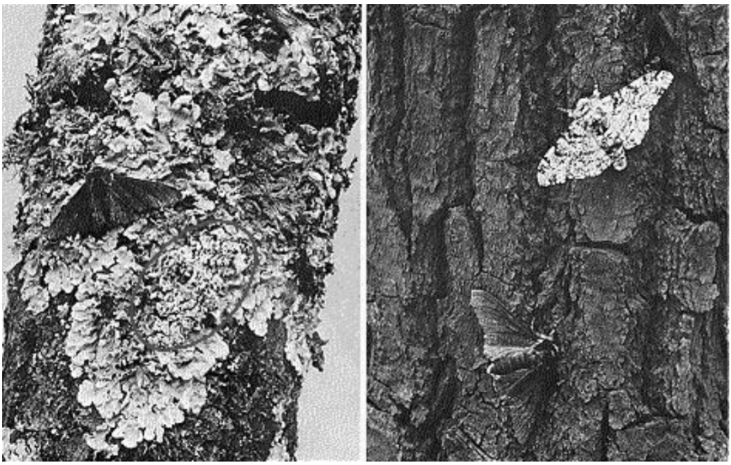
We consider the spread of a favored allele in a diploid population. The classic example - widely repeated in biology textbooks as a modern example of natural selection - is the change in the frequencies of the dark and light phenotypes of the peppered moth during England’s industrial revolution. The evolutionary story begins with the observation that pollution killed the light colored lichen on trees during industrialization of the cities. On the one hand, light colored peppered moths camouflage well on light colored lichens, but are exposed to birds on plain tree bark. On the other hand, dark colored peppered moths camouflage well on plain tree bark, but are exposed on light colored lichens (see Fig. 5.1). Natural selection therefore favored the light-colored allele in preindustrialized England and the dark-colored allele during industrialization. It is believed that the dark-colored allele increased rapidly under natural selection in industrializing England.
We present our model in Table 5.7. Here, we consider aa as the wildtype genotype and normalize its fitness to unity. The allele \(A\) is the mutant whose frequency increases in the population. In our example of the peppered moth, the \(a a\) pheno-
| genotype | \(A A\) | \(A a\) | \(a a\) |
|---|---|---|---|
| freq. of zygote | \(p^{2}\) | \(2 p q\) | \(q^{2}\) |
| relative fitness | \(1+s\) | \(1+s h\) | 1 |
| freq after selection | \((1+s) p^{2} / w\) | \(2(1+s h) p q / w\) | \(q^{2} / w\) |
| normalization | \(w=(1+s) p^{2}+2(1+s h) p q+q^{2}\) |
type is light colored and the \(A A\) phenotype is dark colored. The color of the \(A a\) phenotype depends on the relative dominance of \(A\) and \(a\). Usually, no pigment results in light color and is a consequence of nonfunctioning pigment-producing genes. One functioning pigment-producing allele is usually sufficient to result in a dark-colored moth. With \(A\) a functioning pigment-producing allele and \(a\) the mutated nonfunctioning allele, \(a\) is most likely recessive, \(A\) is most likely dominant, and the phenotype of \(A a\) is most likely dark, so \(h \approx 1\). For the moment, though, we leave \(h\) as a free parameter.
We assume random mating, and this simplification is used to write the genotype frequencies as \(P=p^{2}, Q=2 p q\), and \(R=q^{2}\). Since \(q=1-p\), we reduce our problem to determining an equation for \(p^{\prime}\) in terms of \(p\). Using \(p^{\prime}=P_{s}+(1 / 2) Q_{s}\), where \(p^{\prime}\) is the \(A\) allele frequency in the next generation’s zygotes, and \(P_{S}\) and \(Q_{S}\) are the \(A A\) and \(A a\) genotype frequencies, respectively, in the present generation after selection,
\[p^{\prime}=\frac{(1+s) p^{2}+(1+s h) p q}{w} \nonumber \]
where \(q=1-p\), and
\[\begin{aligned} w &=(1+s) p^{2}+2(1+s h) p q+q^{2} \\[4pt] &=1+s\left(p^{2}+2 h p q\right) \end{aligned} \nonumber \]
After some algebra, the final evolution equation written solely in terms of \(p\) is
\[p^{\prime}=\frac{(1+s h) p+s(1-h) p^{2}}{1+2 s h p+s(1-2 h) p^{2}} \nonumber \]
The expected fixed points of this equation are \(p_{*}=0\) (unstable) and \(p_{*}=1\) (stable), where our assignment of stability assumes positive selection coefficients.
The evolution equation (5.2.9) in this form is not particularly illuminating. In general, a numerical solution would require specifying numerical values for \(s\) and \(h\), as well as an initial value for \(p\). Here, to determine how the spread of \(A\) depends on the dominance coefficient \(h\), we investigate analytically the increase of \(A\) assuming \(s \ll 1\). We Taylor-series expand the right-hand-side of (5.2.9) in powers of \(s\), keeping terms to order \(s\) :
\[\begin{align} \nonumber p^{\prime} &=\frac{(1+s h) p+s(1-h) p^{2}}{1+2 s h p+s(1-2 h) p^{2}} \\[4pt] &=\frac{p+s\left(h p+(1-h) p^{2}\right)}{1+s\left(2 h p+(1-2 h) p^{2}\right)} \\[4pt] &=\left(p+s\left(h p+(1-h) p^{2}\right)\right)\left(1-s\left(2 h p+(1-2 h) p^{2}\right)+\mathrm{O}\left(s^{2}\right)\right)\nonumber \\[4pt] &=p+s p\left(h+(1-3 h) p-(1-2 h) p^{2}\right)+\mathrm{O}\left(s^{2}\right)\nonumber \end{align} \nonumber \]
| disease | mutation | symptoms |
|---|---|---|
| Thalassemia | haemoglobin | anemia |
| Sickle cell anemia | haemoglobin | anemia |
| Haemophilia | blood clotting factor | uncontrolled bleeding |
| Cystic Fibrosis | chloride ion channel | thick lung mucous |
| Tay-Sachs disease | Hexosaminidase A enzyme | nerve cell damage |
| Fragile X syndrome | FMR1 gene | mental retardation |
| Huntington’s disease | HD gene | brain degeneration |
If \(s \ll 1\), we expect a small change in allele frequency in each generation, so we can approximate \(p^{\prime}-p \approx d p / d n\), where \(n\) denotes the generation number, and \(p=p(n) .\) The approximate differential equation obtained from (5.2.10) is
\[\frac{d p}{d n}=s p\left(h+(1-3 h) p-(1-2 h) p^{2}\right) \nonumber \]
If \(A\) is partially dominant so that \(h \neq 0(e . g .\), the heterozygous moth is darker than the homozgygous mutant moth), then the solution to (5.2.11) behaves similarly to the solution of a logistic equation: \(p\) initially grows exponentially as \(p(n)=\) \(p_{0} \exp (s h n)\), and asymptotes to one for large \(n .\) If \(A\) is recessive so that \(h=0(e . g .,\), the heterozygous moth is as light-colored as the homozygous mutant moth), then (5.2.11) reduces to
\[\frac{d p}{d n}=s p^{2}(1-p), \quad \text { for } h=0 \nonumber \]
Of main interest is the initial growth of \(p\) when \(p(0)=p_{0} \ll 1\), so that \(d p / d n \approx s p^{2}\). This differential equation may be integrated by separating variables to yield
\[\begin{aligned} p(n) &=\frac{p_{0}}{1-s p_{0} n} \\[4pt] & \approx p_{0}\left(1+s p_{0} n\right) \end{aligned} \nonumber \]
The frequency of a recessive favored allele increases only linearly across generations, a consequence of the heterozygote being hidden from natural selection. Most likely, the peppered-moth heterozygote is significantly darker than the light-colored homozygote since the dark colored moth rapidly increased in frequency over a short period of time.
As a final comment, linear growth in the frequency of \(A\) when \(h=0\) is sensitive to our assumption of random mating. If selfing occurred, or another type of close family mating, then a recessive favored allele may still increase exponentially. In this circumstance, the production of homozygous offspring from more frequent heterozygote pairings allows selection to act more effectively.
Mutation-selection balance
By virtue of self-knowledge, the species with the most known mutant phenotypes is Homo sapiens. There are thousands of known genetic diseases in humans, many of them caused by mutation of a single gene (called a monogenic disease). For an easy-to-read overview of genetic disease in humans, see the website
http://www.who.int/genomics/public/geneticdiseases
| genotype | \(A A\) | \(A a\) | \(a a\) |
|---|---|---|---|
| freq. of zygote | \(p^{2}\) | \(2 p q\) | \(q^{2}\) |
| relative fitness | 1 | \(1-s h\) | \(1-s\) |
| freq after selection | \(p^{2} / w\) | \(2(1-s h) p q / w\) | \((1-s) q^{2} / w\) |
| normalization | \(w=p^{2}+2(1-s h) p q+(1-s) q^{2}\) |
Table \(5.8\) lists seven common monogenic diseases. The first two diseases are maintained at significant frequencies in some human populations by heterosis. We will discuss in \(\$ 5.2 .4\) the maintenance of a polymorphism by heterosis, for which the heterozygote has higher fitness than either homozygote. It is postulated that Tay-Sachs disease, prevalent among ancestors of Eastern European Jews, and cystic fibrosis may also have been maintained by heterosis acting in the past. (Note that the cystic fibrosis gene was identified in 1989 by a Toronto group led by Lap Chee Tsui, who later became President of the University of Hong Kong.) The other disease genes listed may be maintained by mutation-selection balance.
Our model for diploid mutation-selection balance is given in Table 5.9. We further assume that mutations of type \(A \rightarrow\) a occur in gamete production with frequency \(u\). Back-mutation is neglected. The gametic frequency of \(A\) and \(a\) after selection but before mutation is given by \(\hat{p}=P_{s}+Q_{s} / 2\) and \(\hat{q}=R_{s}+Q_{s} / 2\), and the gametic frequency of \(a\) after mutation is given by \(q^{\prime}=u \hat{p}+\hat{q} .\) Therefore,
\[q^{\prime}=\left(u\left(p^{2}+(1-s h) p q\right)+\left((1-s) q^{2}+(1-s h) p q\right)\right) / w \nonumber \]
where
\[\begin{aligned} w &=p^{2}+2(1-s h) p q+(1-s) q^{2} \\[4pt] &=1-s q(2 h p+q) \end{aligned} \nonumber \]
Using \(p=1-q\), we write the evolution equation for \(q^{\prime}\) in terms of \(q\) alone. After some algebra that could be facilitated using a computer algebra software such as Mathematica, we obtain
\[q^{\prime}=\frac{u+(1-u-\operatorname{sh}(1+u)) q-s(1-h(1+u)) q^{2}}{1-2 \operatorname{sh} q-s(1-2 h) q^{2}} \nonumber \]
To determine the equilibrium solutions of \((5.2.14)\), we set \(q_{*} \equiv q^{\prime}=q\) to obtain a cubic equation for \(q_{*}\). Because of the neglect of back mutation in our model, one solution readily found is \(q_{*}=1\), in which all the \(A\) alleles have mutated to a. The \(q_{*}=1\) solution may be factored out of the cubic equation resulting in a quadratic equation, with two solutions. Rather than show the exact result here, we determine equilibrium solutions under two approximations: (i) \(0<u \ll h, s\), and; (ii) \(0=h<u<s\).
First, when \(0<u \ll h, s\), we look for a solution of the form \(q_{*}=a u+\mathrm{O}\left(u^{2}\right)\), with \(a\) constant, and Taylor series expand in \(u\) (assuming \(\left.s, h=\mathrm{O}\left(u^{0}\right)\right)\). If such a solution exists, then \((5.2.14)\) will determine the unknown coefficient \(a\). We have
\[\begin{aligned} a u+\mathrm{O}\left(u^{2}\right) &=\frac{u+(1-\operatorname{sh}) a u+\mathrm{O}\left(u^{2}\right)}{1-2 \operatorname{shau}+\mathrm{O}\left(u^{2}\right)} \\[4pt] &=(1+a-\operatorname{sh} a) u+\mathrm{O}\left(u^{2}\right) \end{aligned} \nonumber \]
| genotype | \(A A\) | \(A a\) | \(a a\) |
|---|---|---|---|
| freq: \(0<u \ll s, h\) | \(1+\mathrm{O}(u)\) | \(2 u / s h+\mathrm{O}\left(u^{2}\right)\) | \(u^{2} /(s h)^{2}+\mathrm{O}\left(u^{3}\right)\) |
| freq: \(0=h<u<s\) | \(1+\mathrm{O}(\sqrt{u})\) | \(2 \sqrt{u / s}+\mathrm{O}(u)\) | \(u / s\) |
and equating powers of \(u\), we find \(a=1+a-\operatorname{sh} a\), or \(a=1 / \mathrm{sh} .\) Therefore,
\[q_{*}=u / s h+\mathrm{O}\left(u^{2}\right), \quad \text { for } 0<u \ll h, s . \nonumber \]
Second, when \(0=h<u<s\), we substitute \(h=0\) directly into (5.2.14),
\[q_{*}=\frac{u+(1-u) q_{*}-s q_{*}^{2}}{1-s q_{*}^{2}} \nonumber \]
which we then write as a cubic equation \(q_{*}\)
\[q_{*}^{3}-q_{*}^{2}-\frac{u}{s} q_{*}+\frac{u}{s}=0 \nonumber \]
By factoring this cubic equation, we find
\[\left(q_{*}-1\right)\left(q_{*}^{2}-u / s\right)=0 \nonumber \]
and the polymorphic equilibrium solution is
\[q_{*}=\sqrt{u / s}, \quad \text { for } 0=h<u<s \nonumber \]
Because \(q_{*}<1\) only if \(s>u\), this solution does not exist if \(s<u .\)
Table \(5.10\) summarizes our results for the equilibrium frequencies of the genotypes at mutation-selection balance. The first row of frequencies, \(0<u \ll s, h\), corresponds to a dominant \((h=1)\) or partially-dominant \((u \ll h<1)\) mutation, where the heterozygote is of reduced fitness and shows symptoms of the genetic disease. The second row of frequencies, \(0=h<u<s\), corresponds to a recessive mutation, where the heterozygote is symptom-free. Notice that individuals carrying a dominant mutation are twice as prevalent in the population as individuals homozygous for a recessive mutation (with the same \(u\) and \(s\) ).
A heterozygote carrying a dominant mutation most commonly arises either de novo (by direct mutation of allele \(A\) ) or by the mating of a heterozygote with a wildtype. The latter is more common for \(s \ll 1\), while the former must occur for \(s=1\) (a heterozygote with an \(s=h=1\) mutation by definition does not reproduce). One of the most common autosomal dominant genetic diseases is Huntington’s disease, resulting in brain deterioration during middle age. Because individuals with Huntington’s disease have children before disease symptoms appear, \(s\) is small and the disease is usually passed to offspring by the mating of a (heterozygote) with a wildtype homozygote. For a recessive mutation, a mutant homozygote usually occurs by the mating of two heterozygotes. If both parents carry a single recessive disease allele, then their child has a \(1 / 4\) chance of getting the disease.
Heterosis
Heterosis, also called overdominance or heterozygote advantage, occurs when the heterozygote has higher fitness than either homozygote. The best-known examples
| genotype | \(A A\) | \(A a\) | \(a a\) |
|---|---|---|---|
| freq. of zygote | \(p^{2}\) | \(2 p q\) | \(q^{2}\) |
| relative fitness | \(1-s\) | 1 | \(1-t\) |
| freq after selection | \((1-s) p^{2} / w\) | \(2 p q / w\) | \((1-t) q^{2} / w\) |
| normalization | \(w=(1-s) p^{2}+2 p q+(1-t) q^{2}\) |
are sickle-cell anemia and thalassemia, diseases that both affect hemoglobin, the oxygen-carrier protein of red blood cells. The sickle-cell mutations are most common in people of West African descent, while the thalassemia mutations are most common in people from the Mediterranean and Asia. In Hong Kong, the television stations occasionally play public service announcements concerning thalassemia. The heterozygote carrier of the sickle-cell or thalassemia gene is healthy and resistant to malaria; the wildtype homozygote is healthy, but susceptible to malaria; the mutant homozygote is sick with anemia. In class, we will watch the short video, \(A\) Mutation Story, about the sickle cell gene.
Table \(5.11\) presents our model of heterosis. Both homozygotes are of lower fitness than the heterozygote, whose relative fitness we arbitrarily set to unity. Writing the equation for \(p^{\prime}\), we have
\[\begin{aligned} p^{\prime} &=\frac{(1-s) p^{2}+p q}{1-s p^{2}-t q^{2}} \\[4pt] &=\frac{p-s p^{2}}{1-t+2 t p-(s+t) p^{2}} \end{aligned} \nonumber \]
At equilibrium, \(p_{*} \equiv p^{\prime}=p\), and we obtain a cubic equation for \(p_{*}:\)
\[(s+t) p_{*}^{3}-(s+2 t) p_{*}^{2}+t p_{*}=0 \nonumber \]
Evidently, \(p_{*}=0\) and \(p_{*}=1\) are fixed points, and (5.2.20) can be factored as
\[p(1-p)(t-(s+t) p)=0 \nonumber \]
The polymorphic solution is therefore
\[p_{*}=\frac{t}{s+t}, \quad q_{*}=\frac{s}{s+t}, \nonumber \]
valid when \(s, t>0\). Since the value of \(q_{*}\) can be large, recessive mutations that cause disease, yet are highly prevalent in a population, are suspected to provide some benefit to the heterozygote. However, only a few genes are unequivocally known to exhibit heterosis.