5.4: Linkage Equilibrium

When considering a polymorphism at a single genetic locus, we assumed two distinct alleles, \(A\) and \(a\). The diploid then occurs as one of three types: \(A A, A a\) and aa. We now consider a polymorphism at two genetic loci, each with two distinct alleles. If the alleles at the first genetic loci are \(A\) and \(a\), and those at the second \(B\) and \(b\), then four distinct haploid gametes are possible, namely \(A B, A b, a B\) and \(a b\). Ten distinct diplotypes are possible, obtained by forming pairs of all possible haplotypes. We can write these ten diplotypes as \(A B / A B, A B / A b, A B / a B, A B / a b\), \(A b / A b, A b / a B, A b / a b, a B / a B, a B / a b\), and \(a b / a b\), where the numerator represents the haplotype from one parent, the denominator represents the haplotype from the other parent. We do not distinguish here which haplotype came from which parent.

To proceed further, we define the allelic and gametic frequencies for our two loci problem in Table 5.13. If the probability that a gamete contains allele \(A\) or \(a\) does not depend on whether the gamete contains allele \(B\) or \(b\), then the two loci are said to be independent. Under the assumption of independence, the gametic frequencies are the products of the allelic frequencies, i.e., \(p_{A B}=p_{A} p_{B}, p_{A b}=p_{A} p_{b}\), etc.

Often, the two loci are not independent. This can be due to epistatic selection, or epistasis. As an example, suppose that two loci in humans influence height, and that the most fit genotype is the one resulting in an average height. Selection that favors the average population value of a trait is called normalizing or stabilizing. Suppose that \(A\) and \(B\) are hypothetical tall alleles, \(a\) and \(b\) are short alleles, and a person with two tall and two short alleles obtains average height. Then selection may favor the specific genotypes \(A B / a b, A b / A b, A b / a B\), and \(a B / a B\). Selection may act against both the genotypes yielding above average heights, \(A B / A B, A B / A b\), and \(A B / a B\), and those yielding below average heights, \(A b / a b, a B / a b\) and \(a b / a b\). Epistatic selection occurs because the fitness of the \(A, a\) loci depends on which alleles are present at the \(B, b\) loci. Here, \(A\) has higher fitness when paired with \(b\) than when paired with \(B\).

The two loci may also not be independent because of a finite population size (i.e., stochastic effects). For instance, suppose a mutation \(a \rightarrow A\) occurs only once in a finite population (in an infinite population, any possible mutation occurs an infinite number of times), and that \(A\) is strongly favored by natural selection. The frequency of \(A\) may then increase. If a nearby polymorphic locus on the same chromosome as \(A\) happens to be \(B\) (say, with a polymorphism \(b\) in the population), then \(A B\) gametes may substantially increase in frequency, with \(A b\) absent. We say that the allele \(B\) hitchhikes with the favored allele \(A\).

When the two loci are not independent, we say that the loci are in gametic phase disequilibrium, or more commonly linkage disequilibrium, sometimes abbreviated as LD. When the loci are independent, we say they are in linkage equilibrium. Here, we will model how two loci, initially in linkage disequilibrium, approach linkage equilibrium through the process of recombination.

To begin, we need a rudimentary understanding of meiosis. During meiosis, a

Table 5.13: Definitions of allelic and gametic frequencies for two genetic loci each with two alleles.

allele or gamete genotype	\(A\)	\(a\)	\(B\)	\(b\)	\(A B\)	\(A b\)	\(a B\)	\(a b\)
frequency	\(p_{A}\)	\(p_{a}\)	\(p_{B}\)	\(p_{b}\)	\(p_{A B}\)	\(p_{A b}\)	\(p_{a B}\)	\(p_{a b}\)

Figure 5.2: A schematic of crossing-over and recombination during meiosis (figure from Access Excellence @ the National Health Museum)

diploid cell’s DNA, arranged in very long molecules called chromosomes, is replicated once and separated twice, producing four haploid cells, each containing half of the original cell’s chromosomes. Sexual reproduction results in syngamy, the fusing of a haploid egg and sperm cell to form a diploid zygote cell.

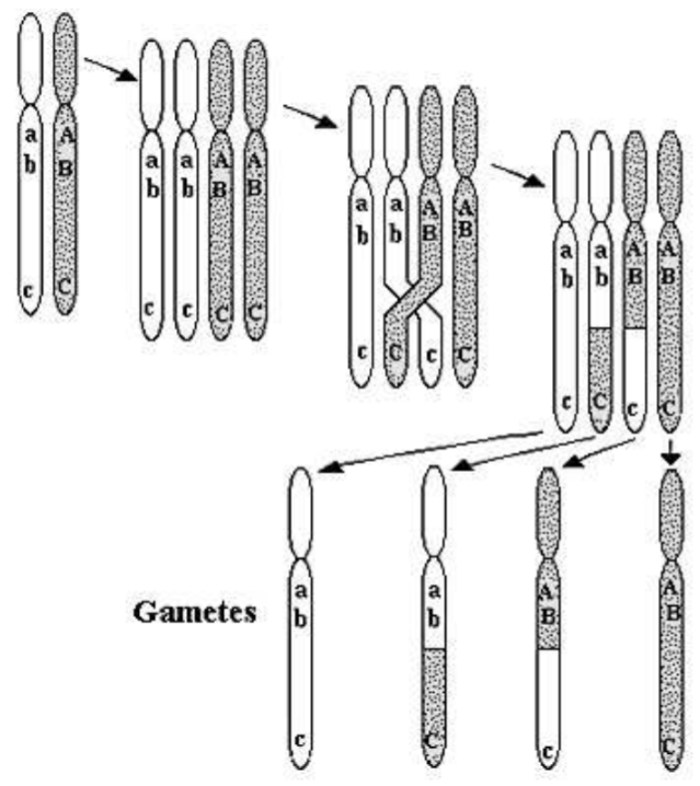
Fig. \(5.2\) presents a schematic of meiosis and the process of crossing-over resulting in recombination. In a diploid, each chromosome has a corresponding sister chromosome, one chromosome originating from the egg, one from the sperm. These sibling chromosomes have the same genes, but possibly different alleles. In Fig. 5.2, we schematically show the alleles \(a, b, c\) on the light chromosome, and the alleles \(A, B, C\) on its sister’s dark chromosome. In the first step of meiosis, each chromosome replicates itself exactly. In the second step, sister chromosomes exchange genetic material by the process of crossing-over. All four chromosomes then separate into haploid cells. Notice from the schematic that the process of crossing-over can result in genetic recombination. Suppose that the schematic of Fig. \(5.2\) represents the production of sperm by a male. If the chromosome from the male’s father contains the alleles \(A B C\) and that from the male’s mother \(a b c\), recombination can result in the sperm containing a chromosome with alleles \(A B c\) (the third gamete in Fig. 5.2). We say this chromosome is a recombinant; it contains alleles from both its paternal grandfather and paternal grandmother. It is likely that the precise combination of alleles on this recombinant chromosome has never existed before in a single person. Recombination is the reason why everybody, with the exception of identical twins, is genetically unique.

Genes that occur on the same chromosome are said to be linked. The closer the genes are to each other on the chromosome, the tighter the linkage, and the less likely recombination will separate them. Tightly linked genes are likely to be inherited from the same grandparent. Genes on different chromosomes are by definition unlinked; independent assortment of chromosomes results in a \(50 \%\) chance of a gamete receiving either grandparents’ genes. To define and model the evolution of linkage disequilibrium, we first obtain allele frequencies from gametic frequencies by

\[\begin{array}{ll} p_{A}=p_{A B}+p_{A b}, & p_{a}=p_{a B}+p_{a b} \\[4pt] p_{B}=p_{A B}+p_{a B}, & p_{b}=p_{A b}+p_{a b} \end{array} \nonumber \]

Since the frequencies sum to unity,

\[p_{A}+p_{a}=1, \quad p_{B}+p_{b}=1, \quad p_{A B}+p_{A b}+p_{a B}+p_{a b}=1 . \nonumber \]

There are three independent gametic frequencies and only two independent allelic frequencies, so in general it is not possible to obtain the gametic frequencies from the allelic frequencies without assuming an additional constraint such as linkage equilibrium. We can, however, introduce an additional variable \(D\), called the coefficient of linkage disequilibrium, and define \(D\) to be the difference between the gametic frequency \(p_{A B}\) and what this gametic frequency would be if the loci were in linkage equilibrium:

\[p_{A B}=p_{A} p_{B}+D \nonumber \]

Using \(p_{A B}+p_{A b}=p_{A}\) to eliminate \(p_{A B}\) in (5.4.3), we obtain

\[p_{A b}=p_{A} p_{b}-D \nonumber \]

Likewise, using \(p_{A B}+p_{a B}=p_{B}\)

\[p_{a B}=p_{a} p_{B}-D \nonumber \]

and using \(p_{a b}+p_{a b}=p_{a}\)

\[p_{a b}=p_{a} p_{b}+D . \nonumber \]

With our definition, positive linkage disequilibrium \((D>0)\) implies excessive \(A B\) and \(a b\) gametes and deficient \(A b\) and \(a B\) gametes; negative linkage disequilibrium \((D<0)\) implies the opposite. \(D\) attains its maximum value of \(1 / 4\) when \(p_{A B}=\) \(p_{a b}=1 / 2\), and attains its minimum value of \(-1 / 4\) when \(p_{A b}=p_{a B}=1 / 2\). An equality obtainable from (5.4.3, 5.4.4, 5.4.5, 5.4.6) that we will later find useful is

\[\begin{align} \nonumber p_{A B} p_{a b}-p_{A b} p_{a B} &=\left(p_{A} p_{B}+D\right)\left(p_{a} p_{b}+D\right)-\left(p_{A} p_{b}-D\right)\left(p_{a} p_{B}-D\right) \\[4pt] \nonumber &=D\left(p_{A} p_{B}+p_{a} p_{b}+p_{A} p_{b}+p_{a} p_{B}\right) \\[4pt] &=D \end{align} \nonumber \]

Without selection and mutation, \(D\) evolves only because of recombination. With primes representing the values in the next generation, and using \(p_{A}^{\prime}=p_{A}\) and \(p_{B}^{\prime}=p_{B}\) because sexual reproduction by itself does not change allele frequencies,

\[\begin{aligned} D^{\prime} &=p_{A B}^{\prime}-p_{A}^{\prime} p_{B}^{\prime} \\[4pt] &=p_{A B}^{\prime}-p_{A} p_{B} \\[4pt] &=p_{A B}^{\prime}-\left(p_{A B}-D\right) \\[4pt] &=D+\left(p_{A B}^{\prime}-p_{A B}\right), \end{aligned} \nonumber \]

where we have used (5.4.3) to obtain the third equality. The change in \(D\) is therefore equal to the change in frequency of the \(A B\) gametes,

\[D^{\prime}-D=p_{A B}^{\prime}-p_{A B} \nonumber \]

Table 5.14: Computation of gamete frequencies.

		gamete freq / diploid freq
diploid	dip freq	AB	Ab	aB	ab
\(A B / A B\)	\(p_{A B}^{2}\)	1	0	0	0
\(A B / A b\)	\(2 p_{A B} p_{A b}\)	\(1 / 2\)	\(1 / 2\)	0	0
\(A B / a B\)	\(2 p_{A B} p_{a B}\)	\(1 / 2\)	0	\(1 / 2\)	0
\(A B / a b\)	\(2 p_{A B} p_{a b}\)	\((1-r) / 2\)	\(r / 2\)	\(r / 2\)	\((1-r) / 2\)
\(A b / A b\)	\(p_{A b}^{2}\)	0	1	0	0
\(A b / a B\)	\(2 p_{A b} p_{a B}\)	\(r / 2\)	\((1-r) / 2\)	\((1-r) / 2\)	\(r / 2\)
\(A b / a b\)	\(2 p_{A b} p_{a b}\)	0	\(1 / 2\)	0	\(1 / 2\)
\(a B / a B\)	\(p_{a B}^{2}\)	0	0	1	0
\(a B / a b\)	\(2 p_{a B} p_{a b}\)	0	0	\(1 / 2\)	\(1 / 2\)
\(a b / a b\)	\(p_{a b}^{2}\)	0	0	0	1

To understand why gametic frequencies change across generations, we should first recognize when they do not change. Without genetic recombination, chromosomes maintain their exact identity across generations. Chromosome frequencies without recombination are therefore constant, and for genetic loci on the same chromosome with alleles \(\mathrm{A}, \mathrm{a}\) and \(\mathrm{B}, \mathrm{b}\), say, \(p_{A B}^{\prime}=p_{A B} .\) In an infinite population without selection or mutation, gametic frequencies change only for genetic loci in linkage disequilibrium on different chromosomes, or for genetic loci in linkage disequilibrium on the same chromosome subjected to genetic recombination.

We will compute the frequency \(p_{A B}^{\prime}\) of \(A B\) gametes in the next generation, given the frequency \(p_{A B}\) of \(A B\) gametes in the present generation, using two different methods. The first method uses a mating table. The second method makes a direct probability argument.

The mating table is shown in Table 5.14. The first column is the parent diplotype before meiosis. The second column is the diplotype frequency assuming random mating. The next four columns are the haploid genotype frequencies (normalized by the corresponding diploid frequencies to simplify the table presentation). Here, we define \(r\) to be the frequency at which the gamete arises from a combination of grandmother and grandfather genes. If the \(A, a\) and \(B, b\) loci occur on the same chromosome, then \(r\) is the recombination frequency due to crossing-over. If the \(\mathrm{A}, \mathrm{a}\) and \(\mathrm{B}, \mathrm{b}\) loci occur on different chromosomes, then because of the independent assortment of chromosomes there is an equal probability that the gamete contains all grandfather or grandmother genes, or contains a combination of grandmother and grandfather genes, so that \(r=1 / 2\). Notice that crossing-over or independent assortment is of importance for those pairs of genes for which the grandfather’s and grandmother’s contribution to the diploid genotype share no common alleles (i.e., \(A B / a b\) and \(A b / a B\) genotypes). The frequency \(p_{A B}^{\prime}\) in the next generation is given by the sum of the \(A B\) column (after multiplication by the diploid frequencies). Therefore,

\[\begin{align} \nonumber p_{A B}^{\prime} &=p_{A B}^{2}+p_{A B} p_{A b}+p_{A B} p_{a B}+(1-r) p_{A B} p_{a b}+r p_{A b} p_{a B} \\[4pt] \nonumber &=p_{A B}\left(p_{A B}+p_{A b}+p_{a B}+p_{a b}\right)+r\left(p_{A b} p_{a B}-p_{A B} p_{a b}\right) \\[4pt] &=p_{A B}-r D \end{align} \nonumber \]

where the final equality makes use of \((5.4.2)\) and (5.4.7).

The second method for computing \(p_{A B}^{\prime}\) is more direct. An \(A B\) haplotype can arise from a diploid of general type \(A B / X X\) without recombination, or a diploid of type \(A X / X B\) with recombination. Therefore,

\[p_{A B}^{\prime}=(1-r) p_{A B}+r p_{A} p_{B} \nonumber \]

where the first term is from non-recombinants and the second term from recombinants. With \(p_{A} p_{B}=p_{A B}-D\), we have

\[\begin{aligned} p_{A B}^{\prime} &=(1-r) p_{A B}+r\left(p_{A B}-D\right) \\[4pt] &=p_{A B}-r D \end{aligned} \nonumber \]

the same result as \((5.4.9)\).

Using \((5.4.8)\) and \((5.4.9)\), we derive

\[D^{\prime}=(1-r) D, \nonumber \]

with the solution

\[D_{n}=D_{0}(1-r)^{n} \nonumber \]

Recombination decreases linkage disequilibrium in each generation by a factor of \((1-r)\). Tightly linked genes on the same chromosome have small values of \(r\); unlinked genes on different chromosomes have \(r=1 / 2\). For unlinked genes, linkage disequilibrium decreases by a factor of two in each generation. We conclude that very strong selection is required to maintain linkage disequilibrium for genes on different chromosomes, while weak selection can maintain linkage disequilibrium for tightly linked genes.