6.3: Competitive Inhibition
- Page ID
- 93518
\( \newcommand{\vecs}[1]{\overset { \scriptstyle \rightharpoonup} {\mathbf{#1}} } \)
\( \newcommand{\vecd}[1]{\overset{-\!-\!\rightharpoonup}{\vphantom{a}\smash {#1}}} \)
\( \newcommand{\dsum}{\displaystyle\sum\limits} \)
\( \newcommand{\dint}{\displaystyle\int\limits} \)
\( \newcommand{\dlim}{\displaystyle\lim\limits} \)
\( \newcommand{\id}{\mathrm{id}}\) \( \newcommand{\Span}{\mathrm{span}}\)
( \newcommand{\kernel}{\mathrm{null}\,}\) \( \newcommand{\range}{\mathrm{range}\,}\)
\( \newcommand{\RealPart}{\mathrm{Re}}\) \( \newcommand{\ImaginaryPart}{\mathrm{Im}}\)
\( \newcommand{\Argument}{\mathrm{Arg}}\) \( \newcommand{\norm}[1]{\| #1 \|}\)
\( \newcommand{\inner}[2]{\langle #1, #2 \rangle}\)
\( \newcommand{\Span}{\mathrm{span}}\)
\( \newcommand{\id}{\mathrm{id}}\)
\( \newcommand{\Span}{\mathrm{span}}\)
\( \newcommand{\kernel}{\mathrm{null}\,}\)
\( \newcommand{\range}{\mathrm{range}\,}\)
\( \newcommand{\RealPart}{\mathrm{Re}}\)
\( \newcommand{\ImaginaryPart}{\mathrm{Im}}\)
\( \newcommand{\Argument}{\mathrm{Arg}}\)
\( \newcommand{\norm}[1]{\| #1 \|}\)
\( \newcommand{\inner}[2]{\langle #1, #2 \rangle}\)
\( \newcommand{\Span}{\mathrm{span}}\) \( \newcommand{\AA}{\unicode[.8,0]{x212B}}\)
\( \newcommand{\vectorA}[1]{\vec{#1}} % arrow\)
\( \newcommand{\vectorAt}[1]{\vec{\text{#1}}} % arrow\)
\( \newcommand{\vectorB}[1]{\overset { \scriptstyle \rightharpoonup} {\mathbf{#1}} } \)
\( \newcommand{\vectorC}[1]{\textbf{#1}} \)
\( \newcommand{\vectorD}[1]{\overrightarrow{#1}} \)
\( \newcommand{\vectorDt}[1]{\overrightarrow{\text{#1}}} \)
\( \newcommand{\vectE}[1]{\overset{-\!-\!\rightharpoonup}{\vphantom{a}\smash{\mathbf {#1}}}} \)
\( \newcommand{\vecs}[1]{\overset { \scriptstyle \rightharpoonup} {\mathbf{#1}} } \)
\(\newcommand{\longvect}{\overrightarrow}\)
\( \newcommand{\vecd}[1]{\overset{-\!-\!\rightharpoonup}{\vphantom{a}\smash {#1}}} \)
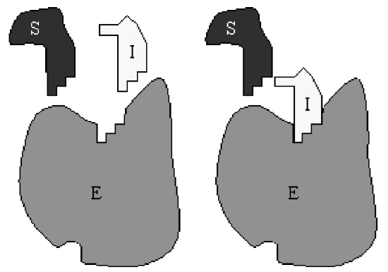
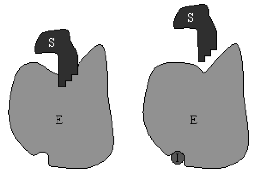
\(\newcommand{\avec}{\mathbf a}\) \(\newcommand{\bvec}{\mathbf b}\) \(\newcommand{\cvec}{\mathbf c}\) \(\newcommand{\dvec}{\mathbf d}\) \(\newcommand{\dtil}{\widetilde{\mathbf d}}\) \(\newcommand{\evec}{\mathbf e}\) \(\newcommand{\fvec}{\mathbf f}\) \(\newcommand{\nvec}{\mathbf n}\) \(\newcommand{\pvec}{\mathbf p}\) \(\newcommand{\qvec}{\mathbf q}\) \(\newcommand{\svec}{\mathbf s}\) \(\newcommand{\tvec}{\mathbf t}\) \(\newcommand{\uvec}{\mathbf u}\) \(\newcommand{\vvec}{\mathbf v}\) \(\newcommand{\wvec}{\mathbf w}\) \(\newcommand{\xvec}{\mathbf x}\) \(\newcommand{\yvec}{\mathbf y}\) \(\newcommand{\zvec}{\mathbf z}\) \(\newcommand{\rvec}{\mathbf r}\) \(\newcommand{\mvec}{\mathbf m}\) \(\newcommand{\zerovec}{\mathbf 0}\) \(\newcommand{\onevec}{\mathbf 1}\) \(\newcommand{\real}{\mathbb R}\) \(\newcommand{\twovec}[2]{\left[\begin{array}{r}#1 \\ #2 \end{array}\right]}\) \(\newcommand{\ctwovec}[2]{\left[\begin{array}{c}#1 \\ #2 \end{array}\right]}\) \(\newcommand{\threevec}[3]{\left[\begin{array}{r}#1 \\ #2 \\ #3 \end{array}\right]}\) \(\newcommand{\cthreevec}[3]{\left[\begin{array}{c}#1 \\ #2 \\ #3 \end{array}\right]}\) \(\newcommand{\fourvec}[4]{\left[\begin{array}{r}#1 \\ #2 \\ #3 \\ #4 \end{array}\right]}\) \(\newcommand{\cfourvec}[4]{\left[\begin{array}{c}#1 \\ #2 \\ #3 \\ #4 \end{array}\right]}\) \(\newcommand{\fivevec}[5]{\left[\begin{array}{r}#1 \\ #2 \\ #3 \\ #4 \\ #5 \\ \end{array}\right]}\) \(\newcommand{\cfivevec}[5]{\left[\begin{array}{c}#1 \\ #2 \\ #3 \\ #4 \\ #5 \\ \end{array}\right]}\) \(\newcommand{\mattwo}[4]{\left[\begin{array}{rr}#1 \amp #2 \\ #3 \amp #4 \\ \end{array}\right]}\) \(\newcommand{\laspan}[1]{\text{Span}\{#1\}}\) \(\newcommand{\bcal}{\cal B}\) \(\newcommand{\ccal}{\cal C}\) \(\newcommand{\scal}{\cal S}\) \(\newcommand{\wcal}{\cal W}\) \(\newcommand{\ecal}{\cal E}\) \(\newcommand{\coords}[2]{\left\{#1\right\}_{#2}}\) \(\newcommand{\gray}[1]{\color{gray}{#1}}\) \(\newcommand{\lgray}[1]{\color{lightgray}{#1}}\) \(\newcommand{\rank}{\operatorname{rank}}\) \(\newcommand{\row}{\text{Row}}\) \(\newcommand{\col}{\text{Col}}\) \(\renewcommand{\row}{\text{Row}}\) \(\newcommand{\nul}{\text{Nul}}\) \(\newcommand{\var}{\text{Var}}\) \(\newcommand{\corr}{\text{corr}}\) \(\newcommand{\len}[1]{\left|#1\right|}\) \(\newcommand{\bbar}{\overline{\bvec}}\) \(\newcommand{\bhat}{\widehat{\bvec}}\) \(\newcommand{\bperp}{\bvec^\perp}\) \(\newcommand{\xhat}{\widehat{\xvec}}\) \(\newcommand{\vhat}{\widehat{\vvec}}\) \(\newcommand{\uhat}{\widehat{\uvec}}\) \(\newcommand{\what}{\widehat{\wvec}}\) \(\newcommand{\Sighat}{\widehat{\Sigma}}\) \(\newcommand{\lt}{<}\) \(\newcommand{\gt}{>}\) \(\newcommand{\amp}{&}\) \(\definecolor{fillinmathshade}{gray}{0.9}\)Competitive inhibition occurs when inhibitor molecules compete with substrate molecules for binding to the same enzyme’s active site. When an inhibitor is bound to the enzyme, no product is produced so competitive inhibition will reduce the velocity of the reaction. A cartoon of this process is shown in Fig. \(6.2\).
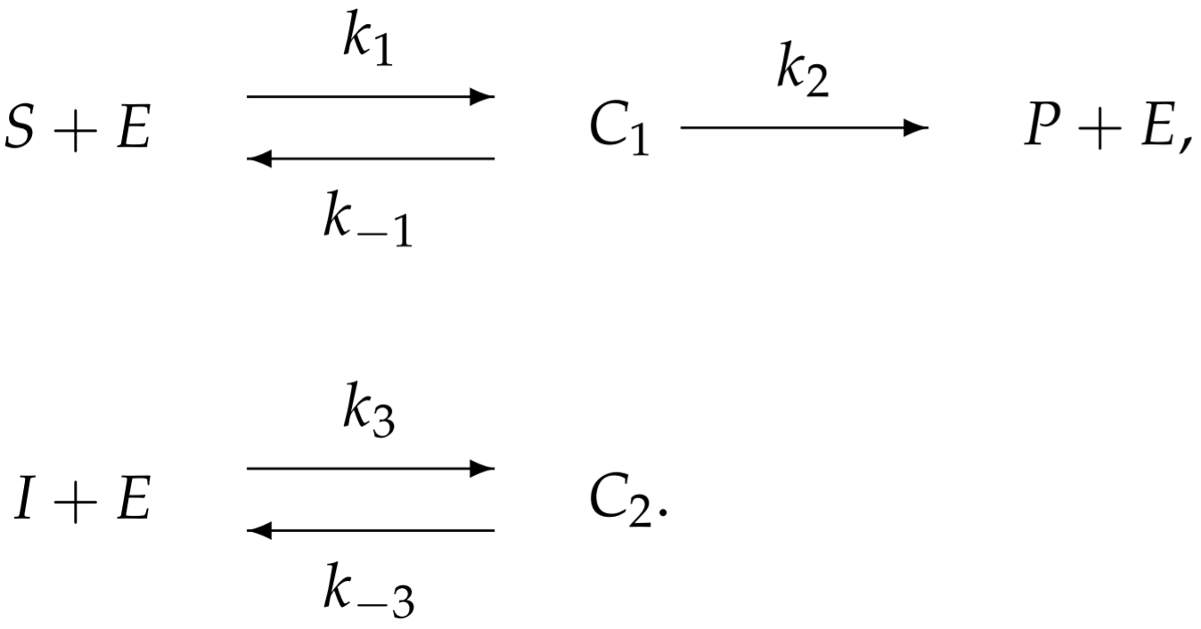
To model competitive inhibition, we introduce an additional reaction associated with the inhibitor-enzyme binding:

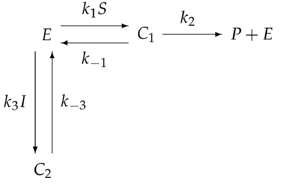
With more complicated enzymatic reactions, the reaction schematic becomes difficult to interpret. Perhaps an easier way to visualize the reaction is from the following redrawn schematic:


Here, the substrate \(S\) and inhibitor \(I\) are combined with the relevant rate constants, rather than treated separately. It is immediately obvious from this redrawn schematic that inhibition is accomplished by sequestering enzyme in the form of \(C_{2}\) and preventing its participation in the catalysis of \(S\) to \(P\).
Our goal is to determine the reaction velocity \(\dot{P}\) in terms of the substrate and inhibitor concentrations, and the total concentration of the enzyme (free and bound). The law of mass action applied to the two complexes and the product results in
\[\begin{aligned} \frac{d C_{1}}{d t} &=k_{1} S E-\left(k_{-1}+k_{2}\right) C_{1} \\[4pt] \frac{d C_{2}}{d t} &=k_{3} I E-k_{-3} C_{2} \\[4pt] \frac{d P}{d t} &=k_{2} C_{1} \end{aligned} \nonumber \]
The enzyme, free and bound, is conserved so that
\[\frac{d}{d t}\left(E+C_{1}+C_{2}\right)=0 \quad \Longrightarrow \quad E+C_{1}+C_{2}=E_{0} \quad \Longrightarrow \quad E=E_{0}-C_{1}-C_{2} . \nonumber \]
Under the quasi-equilibrium approximation, \(C_{1}=\dot{C}_{2}=0\), so that
\[\begin{array}{r} k_{1} S\left(E_{0}-C_{1}-C_{2}\right)-\left(k_{-1}+k_{2}\right) C_{1}=0, \\[4pt] k_{3} I\left(E_{0}-C_{1}-C_{2}\right)-k_{-3} C_{2}=0, \end{array} \nonumber \]
which results in the following system of two linear equations and two unknowns \(\left(C_{1}\right.\) and \(\left.C_{2}\right)\) :
\[\begin{align} \left(k_{-1}+k_{2}+k_{1} S\right) C_{1}+k_{1} S C_{2} &=k_{1} E_{0} S \\[4pt] k_{3} I C_{1}+\left(k_{-3}+k_{3} I\right) C_{2} &=k_{3} E_{0} I \end{align} \nonumber \]
We define the Michaelis-Menten constant \(K_{m}\) as before, and an additional constant \(K_{i}\) associated with the inhibitor reaction:
\[K_{m}=\frac{k_{-1}+k_{2}}{k_{1}}, \quad K_{i}=\frac{k_{-3}}{k_{3}} \nonumber \]
Dividing \((6.3.2)\) by \(k_{1}\) and \((6.3.3)\) by \(k_{3}\) yields
\[\begin{align} \left(K_{m}+S\right) C_{1}+S C_{2} &=E_{0} S \\[4pt] I C_{1}+\left(K_{i}+I\right) C_{2} &=E_{0} I \end{align} \nonumber \]
Since our goal is to obtain the velocity of the reaction, which requires determining \(C_{1}\), we multiply \((6.3.5)\) by \(\left(K_{i}+I\right)\) and \((6.3.6)\) by \(S\), and subtract:
\[\begin{aligned} \left(K_{m}+S\right)\left(K_{i}+I\right) C_{1}+S\left(K_{i}+I\right) C_{2} &=E_{0}\left(K_{i}+I\right) S \\[4pt] S I C_{1}+S\left(K_{i}+I\right) C_{2} &=E_{0} S I \\[4pt] \left(\left(K_{m}+S\right)\left(K_{i}+I\right)-S I\right) C_{1} &=K_{i} E_{0} S \end{aligned} \nonumber \]
or after cancellation and rearrangement
\[\begin{aligned} C_{1} &=\frac{K_{i} E_{0} S}{K_{m} K_{i}+K_{i} S+K_{m} I} \\[4pt] &=\frac{E_{0} S}{K_{m}\left(1+I / K_{i}\right)+S} \end{aligned} \nonumber \]
Therefore, the reaction velocity is given by
\[\begin{align} \frac{d P}{d t} &=\frac{\left(k_{2} E_{0}\right) S}{K_{m}\left(1+I / K_{i}\right)+S} \nonumber \\[4pt] &=\frac{V_{m} S}{K_{m}^{\prime}+S} \end{align} \nonumber \]
where
\[V_{m}=k_{2} E_{0}, \quad K_{m}^{\prime}=K_{m}\left(1+I / K_{i}\right) . \nonumber \]
By comparing the inhibited reaction velocity \((6.3.7)\) and \((6.3.8)\) with the uninhibited reaction velocity \((6.2.6)\) and \((6.2.7)\), we observe that inhibition increases the Michaelis-Menten constant of the reaction, but leaves unchanged the maximum reaction velocity. Since the Michaelis-Menten constant is defined as the substrate concentration required to attain one-half of the maximum reaction velocity, addition of an inhibitor with a fixed substrate concentration acts to decrease the reaction velocity. However, a reaction saturated with substrate still attains the uninhibited maximum reaction velocity.


