
10.3: The Dot Product
- Page ID
- 4215

\( \newcommand{\vecs}[1]{\overset { \scriptstyle \rightharpoonup} {\mathbf{#1}} } \)
\( \newcommand{\vecd}[1]{\overset{-\!-\!\rightharpoonup}{\vphantom{a}\smash {#1}}} \)
\( \newcommand{\dsum}{\displaystyle\sum\limits} \)
\( \newcommand{\dint}{\displaystyle\int\limits} \)
\( \newcommand{\dlim}{\displaystyle\lim\limits} \)
\( \newcommand{\id}{\mathrm{id}}\) \( \newcommand{\Span}{\mathrm{span}}\)
( \newcommand{\kernel}{\mathrm{null}\,}\) \( \newcommand{\range}{\mathrm{range}\,}\)
\( \newcommand{\RealPart}{\mathrm{Re}}\) \( \newcommand{\ImaginaryPart}{\mathrm{Im}}\)
\( \newcommand{\Argument}{\mathrm{Arg}}\) \( \newcommand{\norm}[1]{\| #1 \|}\)
\( \newcommand{\inner}[2]{\langle #1, #2 \rangle}\)
\( \newcommand{\Span}{\mathrm{span}}\)
\( \newcommand{\id}{\mathrm{id}}\)
\( \newcommand{\Span}{\mathrm{span}}\)
\( \newcommand{\kernel}{\mathrm{null}\,}\)
\( \newcommand{\range}{\mathrm{range}\,}\)
\( \newcommand{\RealPart}{\mathrm{Re}}\)
\( \newcommand{\ImaginaryPart}{\mathrm{Im}}\)
\( \newcommand{\Argument}{\mathrm{Arg}}\)
\( \newcommand{\norm}[1]{\| #1 \|}\)
\( \newcommand{\inner}[2]{\langle #1, #2 \rangle}\)
\( \newcommand{\Span}{\mathrm{span}}\) \( \newcommand{\AA}{\unicode[.8,0]{x212B}}\)
\( \newcommand{\vectorA}[1]{\vec{#1}} % arrow\)
\( \newcommand{\vectorAt}[1]{\vec{\text{#1}}} % arrow\)
\( \newcommand{\vectorB}[1]{\overset { \scriptstyle \rightharpoonup} {\mathbf{#1}} } \)
\( \newcommand{\vectorC}[1]{\textbf{#1}} \)
\( \newcommand{\vectorD}[1]{\overrightarrow{#1}} \)
\( \newcommand{\vectorDt}[1]{\overrightarrow{\text{#1}}} \)
\( \newcommand{\vectE}[1]{\overset{-\!-\!\rightharpoonup}{\vphantom{a}\smash{\mathbf {#1}}}} \)
\( \newcommand{\vecs}[1]{\overset { \scriptstyle \rightharpoonup} {\mathbf{#1}} } \)
\(\newcommand{\longvect}{\overrightarrow}\)
\( \newcommand{\vecd}[1]{\overset{-\!-\!\rightharpoonup}{\vphantom{a}\smash {#1}}} \)
\(\newcommand{\avec}{\mathbf a}\) \(\newcommand{\bvec}{\mathbf b}\) \(\newcommand{\cvec}{\mathbf c}\) \(\newcommand{\dvec}{\mathbf d}\) \(\newcommand{\dtil}{\widetilde{\mathbf d}}\) \(\newcommand{\evec}{\mathbf e}\) \(\newcommand{\fvec}{\mathbf f}\) \(\newcommand{\nvec}{\mathbf n}\) \(\newcommand{\pvec}{\mathbf p}\) \(\newcommand{\qvec}{\mathbf q}\) \(\newcommand{\svec}{\mathbf s}\) \(\newcommand{\tvec}{\mathbf t}\) \(\newcommand{\uvec}{\mathbf u}\) \(\newcommand{\vvec}{\mathbf v}\) \(\newcommand{\wvec}{\mathbf w}\) \(\newcommand{\xvec}{\mathbf x}\) \(\newcommand{\yvec}{\mathbf y}\) \(\newcommand{\zvec}{\mathbf z}\) \(\newcommand{\rvec}{\mathbf r}\) \(\newcommand{\mvec}{\mathbf m}\) \(\newcommand{\zerovec}{\mathbf 0}\) \(\newcommand{\onevec}{\mathbf 1}\) \(\newcommand{\real}{\mathbb R}\) \(\newcommand{\twovec}[2]{\left[\begin{array}{r}#1 \\ #2 \end{array}\right]}\) \(\newcommand{\ctwovec}[2]{\left[\begin{array}{c}#1 \\ #2 \end{array}\right]}\) \(\newcommand{\threevec}[3]{\left[\begin{array}{r}#1 \\ #2 \\ #3 \end{array}\right]}\) \(\newcommand{\cthreevec}[3]{\left[\begin{array}{c}#1 \\ #2 \\ #3 \end{array}\right]}\) \(\newcommand{\fourvec}[4]{\left[\begin{array}{r}#1 \\ #2 \\ #3 \\ #4 \end{array}\right]}\) \(\newcommand{\cfourvec}[4]{\left[\begin{array}{c}#1 \\ #2 \\ #3 \\ #4 \end{array}\right]}\) \(\newcommand{\fivevec}[5]{\left[\begin{array}{r}#1 \\ #2 \\ #3 \\ #4 \\ #5 \\ \end{array}\right]}\) \(\newcommand{\cfivevec}[5]{\left[\begin{array}{c}#1 \\ #2 \\ #3 \\ #4 \\ #5 \\ \end{array}\right]}\) \(\newcommand{\mattwo}[4]{\left[\begin{array}{rr}#1 \amp #2 \\ #3 \amp #4 \\ \end{array}\right]}\) \(\newcommand{\laspan}[1]{\text{Span}\{#1\}}\) \(\newcommand{\bcal}{\cal B}\) \(\newcommand{\ccal}{\cal C}\) \(\newcommand{\scal}{\cal S}\) \(\newcommand{\wcal}{\cal W}\) \(\newcommand{\ecal}{\cal E}\) \(\newcommand{\coords}[2]{\left\{#1\right\}_{#2}}\) \(\newcommand{\gray}[1]{\color{gray}{#1}}\) \(\newcommand{\lgray}[1]{\color{lightgray}{#1}}\) \(\newcommand{\rank}{\operatorname{rank}}\) \(\newcommand{\row}{\text{Row}}\) \(\newcommand{\col}{\text{Col}}\) \(\renewcommand{\row}{\text{Row}}\) \(\newcommand{\nul}{\text{Nul}}\) \(\newcommand{\var}{\text{Var}}\) \(\newcommand{\corr}{\text{corr}}\) \(\newcommand{\len}[1]{\left|#1\right|}\) \(\newcommand{\bbar}{\overline{\bvec}}\) \(\newcommand{\bhat}{\widehat{\bvec}}\) \(\newcommand{\bperp}{\bvec^\perp}\) \(\newcommand{\xhat}{\widehat{\xvec}}\) \(\newcommand{\vhat}{\widehat{\vvec}}\) \(\newcommand{\uhat}{\widehat{\uvec}}\) \(\newcommand{\what}{\widehat{\wvec}}\) \(\newcommand{\Sighat}{\widehat{\Sigma}}\) \(\newcommand{\lt}{<}\) \(\newcommand{\gt}{>}\) \(\newcommand{\amp}{&}\) \(\definecolor{fillinmathshade}{gray}{0.9}\)The previous section introduced vectors and described how to add them together and how to multiply them by scalars. This section introduces a multiplication on vectors called the dot product.
Definition 57 Dot Product
- Let \(\vec u = \langle u_1,u_2\rangle \) and \(\vec v = \langle v_1,v_2\rangle \) in \(\mathbb{R}^2\). The dot product of \(\vec u\) and \(\vec v\), denoted \(\vec u \cdot \vec v\), is
\[\vec u \cdot \vec v = u_1v_1+u_2v_2.\] - Let \(\vec u = \langle u_1,u_2,u_3\rangle \) and \(\vec v = \langle v_1,v_2,v_3\rangle \) in \(\mathbb{R}^3\). The dot product of \(\vec u\) and \(\vec v\), denoted \(\vec u \cdot \vec v\), is
\[\vec u \cdot \vec v = u_1v_1+u_2v_2+u_3v_3.\]
Note how this product of vectors returns a scalar, not another vector. We practice evaluating a dot product in the following example, then we will discuss why this product is useful.
Example \(\PageIndex{1}\): Evaluating dot products
- Let \(\vec u=\langle 1,2\rangle \), \(\vec v=\langle 3,-1\rangle \) in \(\mathbb{R}^2\). Find \(\vec u \cdot \vec v\).
- Let \(\vec x = \langle 2,-2,5\rangle \) and \(\vec y = \langle -1, 0, 3\rangle \) in \(\mathbb{R}^3\). Find \(\vec x \cdot \vec y\).
Solution
- Using Definition 57, we have \[\vec u \cdot \vec v = 1(3)+2(-1) = 1.\]
- Using the definition, we have
\[\vec x \cdot \vec y = 2(-1) -2(0) + 5(3) = 13.\]
The dot product, as shown by the preceding example, is very simple to evaluate. It is only the sum of products. While the definition gives no hint as to why we would care about this operation, there is an amazing connection between the dot product and angles formed by the vectors. Before stating this connection, we give a theorem stating some of the properties of the dot product.
THEOREM 85 PROPERTIES OF THE DOT PRODUCT
Let \(\vec u\), \(\vec v\) and \(\vec w\) be vectors in \(\mathbb{R}^2\) or \(\mathbb{R}^3\) and let \(c\) be a scalar.
- \(\vec u \cdot \vec v = \vec v \cdot \vec u\) Commutative Property
- \(\vec u\cdot(\vec v+\vec w) =\vec u \cdot \vec v + \vec u \cdot \vec w\) Distributive Property
- \(c(\vec u \cdot \vec v) = (c\vec u)\cdot \vec v = \vec u \cdot (c\vec v)\)
- \(\vec 0 \cdot \vec v = 0\)
- \(\vec v \cdot \vec v= \norm{\vec v}^2 \)
The last statement of the theorem makes a handy connection between the magnitude of a vector and the dot product with itself.
Our definition and theorem give properties of the dot product, but we are still likely wondering "What does the dot product mean?'' It is helpful to understand that the dot product of a vector with itself is connected to its magnitude.
The next theorem extends this understanding by connecting the dot product to magnitudes and angles. Given vectors \(\vec u\) and \(\vec v\) in the plane, an angle \(\theta\) is clearly formed when \(\vec u\) and \(\vec v\) are drawn with the same initial point as illustrated in Figure 10.29(a). (We always take \(\theta\) to be the angle in \([0,\pi]\) as two angles are actually created.)
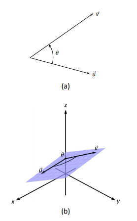
The same is also true of 2 vectors in space: given \(\vec u\) and \(\vec v\) in \(\mathbb{R}^3\) with the same initial point, there is a plane that contains both \(\vec u\) and \(\vec v\). (When \(\vec u\) and \(\vec v\) are co-linear, there are infinite planes that contain both vectors.) In that plane, we can again find an angle \(\theta\) between them (and again, \(0\leq \theta\leq \pi\)). This is illustrated in Figure 10.29(b).
The following theorem connects this angle \(\theta\) to the dot product of \(\vec u\) and \(\vec v\).
theorem 86 the dot product and angles
Let \(\vec u\) and \(\vec v\) be vectors in \(\mathbb{R}^2\) or \(\mathbb{R}^3\). Then
\[\vec u \cdot \vec v = \norm{\vec u}\,\norm{\vec v} \cos\theta,\]
where \(\theta\), \(0\leq\theta\leq \pi\), is the angle between \(\vec u\) and \(\vec v\).
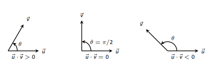
When \(\theta\) is an acute angle (i.e., \(0\leq \theta <\pi/2\)), \(\cos \theta\) is positive; when \(\theta = \pi/2\), \(\cos \theta = 0\); when \(\theta\) is an obtuse angle (\(\pi/2<\theta \leq \pi\)), \(\cos \theta\) is negative. Thus the sign of the dot product gives a general indication of the angle between the vectors, illustrated in Figure 10.30.
We can use Theorem 86 to compute the dot product, but generally this theorem is used to find the angle between known vectors (since the dot product is generally easy to compute). To this end, we rewrite the theorem's equation as
\[\cos \theta = \frac{\vec u \cdot \vec v}{\norm{\vec u}\norm{\vec v}} \quad \Leftrightarrow \quad \theta = \cos^{-1}\left(\frac{\vec u \cdot \vec v}{\norm{\vec u}\norm{\vec v}}\right).\]
We practice using this theorem in the following example.
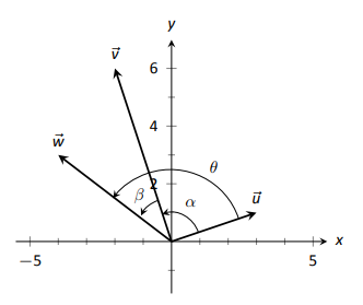
Example \(\PageIndex{2}\): Using the dot product to find angles
Let \(\vec u = \langle 3,1\rangle \), \(\vec v = \langle -2,6\rangle \) and \(\vec w = \langle -4,3\rangle \), as shown in Figure 10.31. Find the angles \(\alpha\), \(\beta\) and \(\theta\).
Solution
We start by computing the magnitude of each vector.
\[\norm{\vec u} = \sqrt{10};\quad \norm{\vec v} = 2\sqrt{10};\quad \norm{\vec w} = 5.\]
We now apply Theorem 86 to find the angles.
\[\begin{align*}
\alpha &= \cos^{-1}\left(\frac{\vec u \cdot \vec v}{(\sqrt{10})(2\sqrt{10})}\right) \\
&= \cos^{-1}(0) = \frac{\pi}2 = 90^\circ. \\
\beta &= \cos^{-1}\left(\frac{\vec v \cdot \vec w}{(2\sqrt{10})(5)}\right) \\
&= \cos^{-1}\left(\frac{26}{10\sqrt{10}}\right) \\
&\approx 0.6055 \approx 34.7^\circ.\\
\theta &= \cos^{-1}\left(\frac{\vec u \cdot \vec w}{(\sqrt{10})(5)}\right) \\
&= \cos^{-1}\left(\frac{-9}{5\sqrt{10}}\right) \\
&\approx 2.1763 \approx 124.7^\circ
\end{align*}\]
We see from our computation that \(\alpha + \beta = \theta\), as indicated by Figure 10.31. While we knew this should be the case, it is nice to see that this non-intuitive formula indeed returns the results we expected.
We do a similar example next in the context of vectors in space.
Example \(\PageIndex{3}\): Using the dot product to find angles
Let \(\vec u = \langle 1,1,1\rangle \), \(\vec v = \langle -1,3,-2\rangle \) and \(\vec w = \langle -5,1,4\rangle \), as illustrated in Figure 10.32. Find the angle between each pair of vectors.
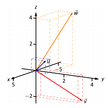
Solution
- Between \(\vec u\) and \(\vec v\):
\[\begin{align*}\theta &= \cos^{-1}\left(\frac{\vec u \cdot \vec v}{\norm{\vec u}\norm{\vec v}}\right)\\&= \cos^{-1}\left(\frac{0}{\sqrt{3}\sqrt{14}}\right)\\&= \frac{\pi}2.\end{align*}\]
- Between \(\vec u\) and \(\vec w\):
\[\begin{align*}\theta &= \cos^{-1}\left(\frac{\vec u \cdot \vec w}{\norm{\vec u}\norm{\vec w}}\right)\\&= \cos^{-1}\left(\frac{0}{\sqrt{3}\sqrt{42}}\right)\\&= \frac{\pi}2.\end{align*}\] - Between \(\vec v\) and \(\vec w\):
\[\begin{align*}\theta &= \cos^{-1}\left(\frac{\vec v \cdot \vec w}{\norm{\vec v}\norm{\vec w}}\right)\\&= \cos^{-1}\left(\frac{0}{\sqrt{14}\sqrt{42}}\right)\\&= \frac{\pi}2.\end{align*}\]
While our work shows that each angle is \(\pi/2\), i.e., \(90^\circ\), none of these angles looks to be a right angle in Figure 10.32. Such is the case when drawing three--dimensional objects on the page.
All three angles between these vectors was \(\pi/2\), or \(90^\circ\). We know from geometry and everyday life that \(90^\circ\) angles are "nice'' for a variety of reasons, so it should seem significant that these angles are all \(\pi/2\). Notice the common feature in each calculation (and also the calculation of \(\alpha\) in Example 10.3.2): the dot products of each pair of angles was 0. We use this as a basis for a definition of the term orthogonal, which is essentially synonymous to perpendicular.
Definition 58 ORTHOGONAL
Vectors \(\vec u\) and \(\vec v\) are orthogonal if their dot product is 0.
Note: The term perpendicular originally referred to lines. As mathematics progressed, the concept of "being at right angles to'' was applied to other objects, such as vectors and planes, and the term orthogonal was introduced. It is especially used when discussing objects that are hard, or impossible, to visualize: two vectors in 5-dimensional space are orthogonal if their dot product is 0. It is not wrong to say they are perpendicular, but common convention gives preference to the word orthogonal.
Example \(\PageIndex{4}\): Finding orthogonal vectors
Let \(\vec u = \langle 3,5\rangle \) and \(\vec v = \langle 1,2,3\rangle \).
- Find two vectors in \(\mathbb{R}^2\) that are orthogonal to \(\vec u\).
- Find two non--parallel vectors in \(\mathbb{R}^3\) that are orthogonal to \(\vec v\).
Solution
- Recall that a line perpendicular to a line with slope \(m\) has slope \(-1/m\), the "opposite reciprocal slope.'' We can think of the slope of \(\vec u\) as \(5/3\), its "rise over run.'' A vector orthogonal to \(\vec u\) will have slope \(-3/5\). There are many such choices, though all parallel:
\[\langle -5,3\rangle \quad \text{or} \quad\langle 5,-3\rangle \quad \text{or} \quad \langle -10,6\rangle \quad \text{or} \quad \langle 15,-9\rangle ,\text{etc.}\]
- There are infinite directions in space orthogonal to any given direction, so there are an infinite number of non--parallel vectors orthogonal to \(\vec v\). Since there are so many, we have great leeway in finding some.
One way is to arbitrarily pick values for the first two components, leaving the third unknown. For instance, let \(\vec v_1 = \langle 2,7,z\rangle \). If \(\vec v_1\) is to be orthogonal to \(\vec v\), then \(\vec v_1\cdot\vec v = 0\), so
\[2+14+3z=0 \quad \Rightarrow z = \frac{-16}{3}.\]
So \(\vec v_1 = \langle 2, 7, -16/3\rangle \) is orthogonal to \(\vec v\). We can apply a similar technique by leaving the first or second component unknown.
Another method of finding a vector orthogonal to \(\vec v\) mirrors what we did in part 1. Let \(\vec v_2 = \langle -2,1,0\rangle \). Here we switched the first two components of \(\vec v\), changing the sign of one of them (similar to the "opposite reciprocal'' concept before). Letting the third component be 0 effectively ignores the third component of \(\vec v\), and it is easy to see that
\[\vec v_2\cdot\vec v = \langle -2,1,0\rangle \cdot\langle 1,2,3\rangle = 0.\]
Clearly \(\vec v_1\) and \(\vec v_2\) are not parallel.
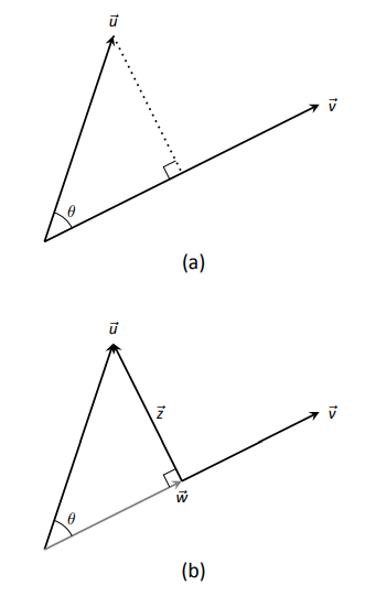
An important construction is illustrated in Figure 10.33, where vectors \(\vec u\) and \(\vec v\) are sketched. In part (a), a dotted line is drawn from the tip of \(\vec u\) to the line containing \(\vec v\), where the dotted line is orthogonal to \(\vec v\). In part (b), the dotted line is replaced with the vector \(\vec z\) and \(\vec w\) is formed, parallel to \(\vec v\). It is clear by the diagram that \(\vec u = \vec w+\vec z\). What is important about this construction is this: \(\vec u\) is decomposed as the sum of two vectors, one of which is parallel to \(\vec v\) and one that is perpendicular to \(\vec v\). It is hard to overstate the importance of this construction (as we'll see in upcoming examples).
The vectors \(\vec w\), \(\vec z\) and \(\vec u\) as shown in Figure 10.33 (b) form a right triangle, where the angle between \(\vec v\) and \(\vec u\) is labeled \(\theta\). We can find \(\vec w\) in terms of \(\vec v\) and \(\vec u\).
Using trigonometry, we can state that
\[\norm{\vec w} = \norm{\vec u}\cos \theta. \label{eq:proj1}\]
We also know that \(\vec w\) is parallel to to \(\vec v\); that is, the direction of \(\vec w\) is the direction of \(\vec v\), described by the unit vector \(\frac{1}{\norm{\vec v}}\vec v\). The vector \(\vec w\) is the vector in the direction \(\frac{1}{\norm{\vec v}}\vec v\) with magnitude \(\norm{\vec u}\cos \theta\):
\[\begin{align*}
\vec w &= \Big(\norm{\vec u}\cos\theta \Big)\frac{1}{\norm{\vec v}}\vec v. \\
\text{Replace \(\cos\theta\) using Theorem 86:}& \\
&= \left(\norm{\vec u}\frac{ \vec u \cdot \vec v }{\norm{\vec u}\norm{\vec v}}\right)\frac{1}{\norm{\vec v}} \vec v\\
&= \frac{ \vec u \cdot \vec v }{\norm{\vec v}^2}\vec v. \\
\text{Now apply Theorem 85.}& \\
&= \frac{\vec u \cdot \vec v}{\vec v \cdot \vec v}\vec v.
\end{align*}\]
Since this construction is so important, it is given a special name.
Definition 59 orthogonal projection
Let \(\vec u\) and \(\vec v\) be given. The orthogonal projection of \(\vec u\) onto \(\vec v\), denoted \(\text{proj}_{\vec v}\vec u\), is
\[\text{proj}_{\vec v}\vec u = \frac{\vec u \cdot \vec v}{\vec v \cdot \vec v}\vec v.\]
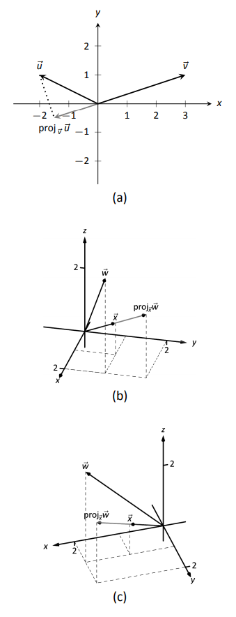
Example \(\PageIndex{5}\): Computing the orthogonal projection
- Let \(\vec u= \langle -2,1\rangle \) and \(\vec v=\langle 3,1\rangle \). Find \(\text{proj}_{\vec v}\vec u\), and sketch all three vectors with initial points at the origin.
- Let \(\vec w = \langle 2,1,3\rangle \) and \(\vec x = \langle 1,1,1\rangle \). Find \(\text{proj}_{\vec x}\vec w\), and sketch all three vectors with initial points at the origin.
Solution
- Applying Definition 59, we have
\[\begin{align*}\text{proj}_{\vec v}\vec u &= \frac{\vec u \cdot \vec v}{\vec v \cdot \vec v}\vec v \\&= \frac{-5}{10}\langle 3,1\rangle \\&= \langle -\frac32,-\frac12\rangle .\end{align*}\]
Vectors \(\vec u\), \(\vec v\) and \(\text{proj}_{\vec v}\vec u\) are sketched in Figure 10.34(a). Note how the projection is parallel to \(\vec v\); that is, it lies on the same line through the origin as \(\vec v\), although it points in the opposite direction. That is because the angle between \(\vec u\) and \(\vec v\) is obtuse (i.e., greater than \(90^\circ\)).
- Apply the definition:
\[\begin{align*}\text{proj}_{\vec x}\vec w &= \frac{\vec w \cdot \vec x}{\vec x \cdot \vec x}\vec x \\&= \frac{6}{3}\langle 1,1,1\rangle \\&= \langle 2,2,2\rangle . \end{align*}\]
These vectors are sketched in Figure 10.34(b), and again in part (c) from a different perspective. Because of the nature of graphing these vectors, the sketch in part (b) makes it difficult to recognize that the drawn projection has the geometric properties it should. The graph shown in part (c) illustrates these properties better.
Consider Figure 10.35 where the concept of the orthogonal projection is again illustrated. It is clear that
\[
\vec u = \text{proj}_{\vec v}\vec u + \vec z.
\label{eq:orthogproj}\]
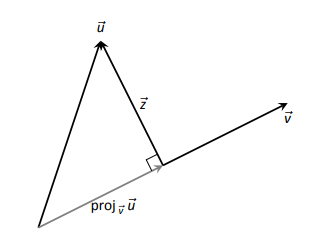
As we know what \(\vec u\) and \(\text{proj}_{\vec v}\vec u\) are, we can solve for \(\vec z\) and state that
\[\vec z = \vec u - \text{proj}_{\vec v}\vec u.\]
This leads us to rewrite Equation \ref{eq:orthogproj} in a seemingly silly way: \[\vec u = \text{proj}_{\vec v}\vec u + (\vec u - \text{proj}_{\vec v}\vec u).\]
This is not nonsense, as pointed out in the following Key Idea. (Notation note: the expression "\(\parallel \vec y\)'' means "is parallel to \(\vec y\).'' We can use this notation to state "\(\vec x\parallel\vec y\)'' which means "\(\vec x\) is parallel to \(\vec y\).'' The expression "\(\perp \vec y\)'' means "is orthogonal to \(\vec y\),'' and is used similarly.)
key idea 49 orthogonal decomposition of vectors
Let \(\vec u\) and \(\vec v\) be given. Then \(\vec u\) can be written as the sum of two vectors, one of which is parallel to \(\vec v\), and one of which is orthogonal to \(\vec v\):
\[\vec u = \underbrace{\text{proj}_{\vec v}\vec u}_{\parallel\ \vec v}\ +\ (\underbrace{\vec u-\text{proj}_{\vec v}\vec u}_{\perp\ \vec v}).\]
We illustrate the use of this equality in the following example.
Example \(\PageIndex{6}\): Orthogonal decomposition of vectors
- Let \(\vec u = \langle -2,1\rangle \) and \(\vec v = \langle 3,1\rangle \) as in Example 10.3.5. Decompose \(\vec u\) as the sum of a vector parallel to \(\vec v\) and a vector orthogonal to \(\vec v\).
- Let \(\vec w =\langle 2,1,3\rangle \) and \(\vec x =\langle 1,1,1\rangle \) as in Example 10.3.5. Decompose \(\vec w\) as the sum of a vector parallel to \(\vec x\) and a vector orthogonal to \(\vec x\).
Solution
- In Example 10.3.5, we found that \(\text{proj}_{\vec v}\vec u = \langle -1.5,-0.5\rangle \). Let \[\vec z = \vec u - \text{proj}_{\vec v}\vec u = \langle -2,1\rangle - \langle -1.5,-0.5\rangle = \langle -0.5, 1.5\rangle .\]
Is \(\vec z\) orthogonal to \(\vec v\)? (I.e, is \(\vec z \perp\vec v\) ?) We check for orthogonality with the dot product:
\[\vec z \cdot \vec v = \langle -0.5,1.5\rangle \cdot \langle 3,1\rangle =0.\]
Since the dot product is 0, we know \(\vec z \perp \vec v\). Thus:
\[\begin{align*}\vec u &= \text{proj}_{\vec v}\vec u\ +\ (\vec u - \text{proj}_{\vec v}\vec u) \\\langle -2,1\rangle &= \underbrace{\langle -1.5,-0.5\rangle }_{\parallel\ \vec v}\ +\ \underbrace{\langle -0.5,1.5\rangle }_{\perp \ \vec v}.\end{align*}\] - We found in Example 10.3.5 that \(\text{proj}_{\vec x}\vec w = \langle 2,2,2\rangle \). Applying the Key Idea, we have:
\[\vec z = \vec w - \text{proj}_{\vec x}\vec w = \langle 2,1,3\rangle - \langle 2,2,2\rangle = \langle 0,-1,1\rangle .\]
We check to see if \(\vec z \perp \vec x\):
\[\vec z \cdot \vec x = \langle 0,-1,1\rangle \cdot \langle 1,1,1\rangle = 0.\]
Since the dot product is 0, we know the two vectors are orthogonal.
We now write \(\vec w\) as the sum of two vectors, one parallel and one orthogonal to \(\vec x\):
\[\begin{align*}\vec w &= \text{proj}_{\vec x}\vec w\ +\ (\vec w - \text{proj}_{\vec x}\vec w) \\\langle 2,1,3\rangle &= \underbrace{\langle 2,2,2\rangle }_{\parallel\ \vec x}\ +\ \underbrace{\langle 0,-1,1\rangle }_{\perp \ \vec x} \end{align*}\]
We give an example of where this decomposition is useful.
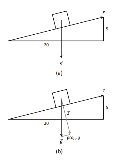
Example \(\PageIndex{7}\): Orthogonally decomposing a force vector
Consider Figure 10.36(a), showing a box weighing 50lb on a ramp that rises 5ft over a span of 20ft. Find the components of force, and their magnitudes, acting on the box (as sketched in part (b) of the figure):
- in the direction of the ramp, and
- orthogonal to the ramp.
Solution
As the ramp rises 5ft over a horizontal distance of 20ft, we can represent the direction of the ramp with the vector \(\vec r= \langle 20,5\rangle \). Gravity pulls down with a force of 50lb, which we represent with \(\vec g = \langle 0,-50\rangle \).
- To find the force of gravity in the direction of the ramp, we compute \(\text{proj}_{\vec r}\vec g\):
\[\begin{align*}\text{proj}_{\vec r}\vec g &= \frac{\vec g \cdot \vec r}{\vec r \cdot \vec r}\vec r\\&= \frac{-250}{425}\langle 20,5\rangle \\&= \langle -\frac{200}{17},-\frac{50}{17}\rangle \approx \langle -11.76,-2.94\rangle .\end{align*}\]
The magnitude of \(\text{proj}_{\vec r}\vec g\) is \(\norm{\text{proj}_{\vec r}\vec g} = 50/\sqrt{17} \approx 12.13\text{lb}\). Though the box weighs 50lb, a force of about 12lb is enough to keep the box from sliding down the ramp.
- To find the component \(\vec z\) of gravity orthogonal to the ramp, we use Key Idea 49.
\[\begin{align*}\vec z &= \vec g - \text{proj}_{\vec r}\vec g \\&= \langle \frac{200}{17},-\frac{800}{17}\rangle \approx \langle 11.76,-47.06\rangle .\end{align*}\]
The magnitude of this force is \(\norm{\vec z} \approx 48.51\)lb. In physics and engineering, knowing this force is important when computing things like static frictional force. (For instance, we could easily compute if the static frictional force alone was enough to keep the box from sliding down the ramp.)
Application to Work
In physics, the application of a force \(F\) to move an object in a straight line a distance \(d\) produces work; the amount of work \(W\) is \(W=Fd\), (where \(F\) is in the direction of travel). The orthogonal projection allows us to compute work when the force is not in the direction of travel.
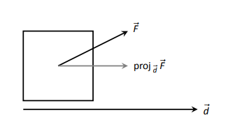
Consider Figure 10.37, where a force \(\vec F\) is being applied to an object moving in the direction of \(\vec d\). (The distance the object travels is the magnitude of \(\vec d\).) The work done is the amount of force in the direction of \(\vec d\), \(\norm{\text{proj}_{\vec d}\vec F}\), times \(\norm d\):
\[\begin{align*}
\norm{\text{proj}_{\vec d}\vec F}\cdot\norm d &= \Big \| \frac{\vec F \cdot \vec d}{\vec d \cdot \vec d}\vec d \Big \| \cdot \norm d \\
&= \left|\frac{\vec F \cdot \vec d}{\norm d^2}\right|\cdot \norm d\cdot\norm d\\
&= \frac{\left|\vec F \cdot \vec d\right|}{\norm d^2}\norm d^2\\
&= \left|\vec F \cdot \vec d\right|.
\end{align*}\]
The expression \(\vec F \cdot \vec d\) will be positive if the angle between \(\vec F\) and \(\vec d\) is acute; when the angle is obtuse (hence \(\vec F \cdot \vec d\) is negative), the force is causing motion in the opposite direction of \(\vec d\), resulting in "negative work.'' We want to capture this sign, so we drop the absolute value and find that \(W = \vec F \cdot \vec d\).
Definition 60 WORK
Let \(\vec F\) be a constant force that moves an object in a straight line from point \(P\) to point \(Q\). Let \(\vec d = \vec{PQ}\). The work \(W\) done by \(\vec F\) along \(\vec d\) is \(W = \vec F \cdot \vec d\).
Example \(\PageIndex{8}\): Computing work
A man slides a box along a ramp that rises 3ft over a distance of 15ft by applying 50lb of force as shown in Figure 10.38. Compute the work done.
Solution
The figure indicates that the force applied makes a \(30^\circ\) angle with the horizontal, so \(\vec F = 50\langle \cos 30^\circ,\sin 30^\circ\rangle \approx \langle 43.3,25\rangle .\) The ramp is represented by \(\vec d = \langle 15,3\rangle \). The work done is simply
\[\vec F \cdot \vec d = 50\langle \cos 30^\circ,\sin 30^\circ\rangle \cdot \langle 15,3\rangle \approx 724.5 \text{ft--lb}.\]
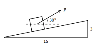
Note how we did not actually compute the distance the object traveled, nor the magnitude of the force in the direction of travel; this is all inherently computed by the dot product!
The dot product is a powerful way of evaluating computations that depend on angles without actually using angles. The next section explores another "product'' on vectors, the cross product. Once again, angles play an important role, though in a much different way.