
4.1: Least Squares
- Page ID
- 21819

\( \newcommand{\vecs}[1]{\overset { \scriptstyle \rightharpoonup} {\mathbf{#1}} } \)
\( \newcommand{\vecd}[1]{\overset{-\!-\!\rightharpoonup}{\vphantom{a}\smash {#1}}} \)
\( \newcommand{\dsum}{\displaystyle\sum\limits} \)
\( \newcommand{\dint}{\displaystyle\int\limits} \)
\( \newcommand{\dlim}{\displaystyle\lim\limits} \)
\( \newcommand{\id}{\mathrm{id}}\) \( \newcommand{\Span}{\mathrm{span}}\)
( \newcommand{\kernel}{\mathrm{null}\,}\) \( \newcommand{\range}{\mathrm{range}\,}\)
\( \newcommand{\RealPart}{\mathrm{Re}}\) \( \newcommand{\ImaginaryPart}{\mathrm{Im}}\)
\( \newcommand{\Argument}{\mathrm{Arg}}\) \( \newcommand{\norm}[1]{\| #1 \|}\)
\( \newcommand{\inner}[2]{\langle #1, #2 \rangle}\)
\( \newcommand{\Span}{\mathrm{span}}\)
\( \newcommand{\id}{\mathrm{id}}\)
\( \newcommand{\Span}{\mathrm{span}}\)
\( \newcommand{\kernel}{\mathrm{null}\,}\)
\( \newcommand{\range}{\mathrm{range}\,}\)
\( \newcommand{\RealPart}{\mathrm{Re}}\)
\( \newcommand{\ImaginaryPart}{\mathrm{Im}}\)
\( \newcommand{\Argument}{\mathrm{Arg}}\)
\( \newcommand{\norm}[1]{\| #1 \|}\)
\( \newcommand{\inner}[2]{\langle #1, #2 \rangle}\)
\( \newcommand{\Span}{\mathrm{span}}\) \( \newcommand{\AA}{\unicode[.8,0]{x212B}}\)
\( \newcommand{\vectorA}[1]{\vec{#1}} % arrow\)
\( \newcommand{\vectorAt}[1]{\vec{\text{#1}}} % arrow\)
\( \newcommand{\vectorB}[1]{\overset { \scriptstyle \rightharpoonup} {\mathbf{#1}} } \)
\( \newcommand{\vectorC}[1]{\textbf{#1}} \)
\( \newcommand{\vectorD}[1]{\overrightarrow{#1}} \)
\( \newcommand{\vectorDt}[1]{\overrightarrow{\text{#1}}} \)
\( \newcommand{\vectE}[1]{\overset{-\!-\!\rightharpoonup}{\vphantom{a}\smash{\mathbf {#1}}}} \)
\( \newcommand{\vecs}[1]{\overset { \scriptstyle \rightharpoonup} {\mathbf{#1}} } \)
\(\newcommand{\longvect}{\overrightarrow}\)
\( \newcommand{\vecd}[1]{\overset{-\!-\!\rightharpoonup}{\vphantom{a}\smash {#1}}} \)
\(\newcommand{\avec}{\mathbf a}\) \(\newcommand{\bvec}{\mathbf b}\) \(\newcommand{\cvec}{\mathbf c}\) \(\newcommand{\dvec}{\mathbf d}\) \(\newcommand{\dtil}{\widetilde{\mathbf d}}\) \(\newcommand{\evec}{\mathbf e}\) \(\newcommand{\fvec}{\mathbf f}\) \(\newcommand{\nvec}{\mathbf n}\) \(\newcommand{\pvec}{\mathbf p}\) \(\newcommand{\qvec}{\mathbf q}\) \(\newcommand{\svec}{\mathbf s}\) \(\newcommand{\tvec}{\mathbf t}\) \(\newcommand{\uvec}{\mathbf u}\) \(\newcommand{\vvec}{\mathbf v}\) \(\newcommand{\wvec}{\mathbf w}\) \(\newcommand{\xvec}{\mathbf x}\) \(\newcommand{\yvec}{\mathbf y}\) \(\newcommand{\zvec}{\mathbf z}\) \(\newcommand{\rvec}{\mathbf r}\) \(\newcommand{\mvec}{\mathbf m}\) \(\newcommand{\zerovec}{\mathbf 0}\) \(\newcommand{\onevec}{\mathbf 1}\) \(\newcommand{\real}{\mathbb R}\) \(\newcommand{\twovec}[2]{\left[\begin{array}{r}#1 \\ #2 \end{array}\right]}\) \(\newcommand{\ctwovec}[2]{\left[\begin{array}{c}#1 \\ #2 \end{array}\right]}\) \(\newcommand{\threevec}[3]{\left[\begin{array}{r}#1 \\ #2 \\ #3 \end{array}\right]}\) \(\newcommand{\cthreevec}[3]{\left[\begin{array}{c}#1 \\ #2 \\ #3 \end{array}\right]}\) \(\newcommand{\fourvec}[4]{\left[\begin{array}{r}#1 \\ #2 \\ #3 \\ #4 \end{array}\right]}\) \(\newcommand{\cfourvec}[4]{\left[\begin{array}{c}#1 \\ #2 \\ #3 \\ #4 \end{array}\right]}\) \(\newcommand{\fivevec}[5]{\left[\begin{array}{r}#1 \\ #2 \\ #3 \\ #4 \\ #5 \\ \end{array}\right]}\) \(\newcommand{\cfivevec}[5]{\left[\begin{array}{c}#1 \\ #2 \\ #3 \\ #4 \\ #5 \\ \end{array}\right]}\) \(\newcommand{\mattwo}[4]{\left[\begin{array}{rr}#1 \amp #2 \\ #3 \amp #4 \\ \end{array}\right]}\) \(\newcommand{\laspan}[1]{\text{Span}\{#1\}}\) \(\newcommand{\bcal}{\cal B}\) \(\newcommand{\ccal}{\cal C}\) \(\newcommand{\scal}{\cal S}\) \(\newcommand{\wcal}{\cal W}\) \(\newcommand{\ecal}{\cal E}\) \(\newcommand{\coords}[2]{\left\{#1\right\}_{#2}}\) \(\newcommand{\gray}[1]{\color{gray}{#1}}\) \(\newcommand{\lgray}[1]{\color{lightgray}{#1}}\) \(\newcommand{\rank}{\operatorname{rank}}\) \(\newcommand{\row}{\text{Row}}\) \(\newcommand{\col}{\text{Col}}\) \(\renewcommand{\row}{\text{Row}}\) \(\newcommand{\nul}{\text{Nul}}\) \(\newcommand{\var}{\text{Var}}\) \(\newcommand{\corr}{\text{corr}}\) \(\newcommand{\len}[1]{\left|#1\right|}\) \(\newcommand{\bbar}{\overline{\bvec}}\) \(\newcommand{\bhat}{\widehat{\bvec}}\) \(\newcommand{\bperp}{\bvec^\perp}\) \(\newcommand{\xhat}{\widehat{\xvec}}\) \(\newcommand{\vhat}{\widehat{\vvec}}\) \(\newcommand{\uhat}{\widehat{\uvec}}\) \(\newcommand{\what}{\widehat{\wvec}}\) \(\newcommand{\Sighat}{\widehat{\Sigma}}\) \(\newcommand{\lt}{<}\) \(\newcommand{\gt}{>}\) \(\newcommand{\amp}{&}\) \(\definecolor{fillinmathshade}{gray}{0.9}\)Introduction
We learned in the previous chapter that \(Ax = b\) need not possess a solution when the number of rows of \(A\) exceeds its rank, i.e., \(r < m\). As this situation arises quite often in practice, typically in the guise of 'more equations than unknowns,' we establish a rationale for the absurdity \(Ax = b\).
The Normal Equations
The goal is to choose \(x\) such that \(Ax\) is as close as possible to \(b\). Measuring closeness in terms of the sum of the squares of the components we arrive at the 'least squares' problem of minimizing
res
\[(||Ax-b||)^2 = (Ax-b)^{T}(Ax-b) \nonumber\]
over all \(x \in \mathbb{R}\). The path to the solution is illuminated by the Fundamental Theorem. More precisely, we write
\(\forall b_{R}, b_{N}, b_{R} \in \mathbb{R}(A) \wedge b_{N} \in \mathbb{N} (A^{T}) : (b = b_{R}+b_{N})\). On noting that (i) \(\forall b_{R}, x \in \mathbb{R}^n : ((Ax-bR) \in \mathbb{R}(A))\) and (ii) \(\mathbb{R}(A) \perp \mathbb{N} (A^T)\) we arrive at the Pythagorean Theorem.
\[norm^{2}(Ax-b) = (||Ax-b_{R}+b_{N}||)^2 \nonumber\]
\[= (||Ax-b_{R}||)^2+(||b_{N}||)^2 \nonumber\]
It is now clear from the Pythagorean Theorem that the best \(x\) is the one that satisfies
\[Ax = b_{R} \nonumber\]
As \(b_{R} \in \mathbb{R}(A)\) this equation indeed possesses a solution. We have yet however to specify how one computes \(b_{R}\) given \(b\). Although an explicit expression for \(b_{R}\) orthogonal projection of \(b\) onto \(\mathbb{R}(A)\), in terms of \(A\) and \(b\) is within our grasp we shall, strictly speaking, not require it. To see this, let us note that if \(x\) satisfies the above equation then orthogonal projection of \(b\) onto \(\mathbb{R}(A)\), in terms of \(A\) and \(b\) is within our grasp we shall, strictly speaking, not require it. To see this, let us note that if \(x\) satisfies the above equation then
\[Ax-b = Ax-b_{R}+b_{N} \nonumber\]
\[= -b_{N} \nonumber\]
As \(b_{N}\) is no more easily computed than \(b_{R}\) you may claim that we are just going in circles. The 'practical' information in the above equation however is that \((Ax-b) \in A^{T}\), i.e., \(A^{T}(Ax-b) = 0\), i.e.,
\[A^{T} Ax = A^{T} b \nonumber\]
As \(A^{T} b \in \mathbb{R} (A^T)\) regardless of \(b\) this system, often referred to as the normal equations, indeed has a solution. This solution is unique so long as the columns of \(A^{T}A\) are linearly independent, i.e., so long as \(\mathbb{N}(A^{T}A) = {0}\). Recalling Chapter 2, Exercise 2, we note that this is equivalent to \(\mathbb{N}(A) = \{0\}\)
The set of \(x \in b_{R}\) for which the misfit \((||Ax-b||)^2\) is smallest is composed of those \(x\) for which \(A^{T}Ax = A^{T}b\) There is always at least one such \(x\). There is exactly one such \(x\) if \(\mathbb{N}(A) = \{0\}\).
As a concrete example, suppose with reference to Figure 1 that \(A = \begin{pmatrix} {1}&{1}\\ {0}&{1}\\ {0}&{0} \end{pmatrix}\) and \(A = \begin{pmatrix} {1}\\ {1}\\ {1} \end{pmatrix}\)
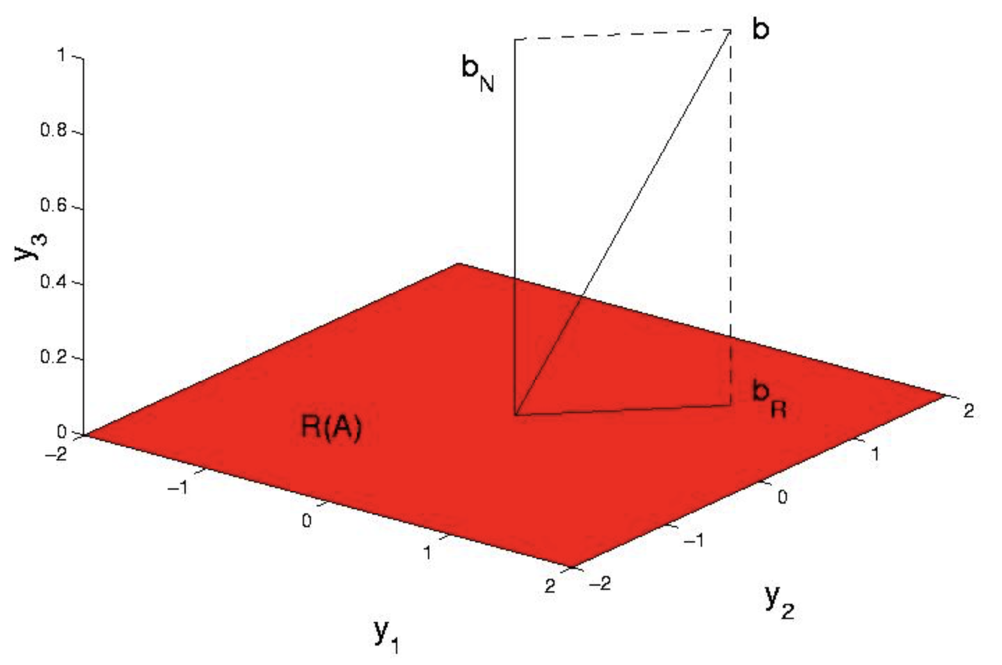
As \(b \ne \mathbb{R}(A)\) there is no \(x\) such that \(Ax = b\). Indeed, \((||Ax-b||)^2 = (x_{1}+x_{2}+-1)^2+(x_{2}-1)^2+1 \ge 1\), with the minimum uniquely attained at \(x = \begin{pmatrix} {0}\\ {1} \end{pmatrix}\), in agreement with the unique solution of the above equation, for \(A^{T} A = \begin{pmatrix} {1}&{1}\\ {1}&{2} \end{pmatrix}\) and \(A^{T} b = \begin{pmatrix} {1}\\ {2} \end{pmatrix}\). We now recognize, a posteriori, that \(b_{R} = Ax = \begin{pmatrix} {1}\\ {1}\\ {0} \end{pmatrix}\) is the orthogonal projection of b onto the column space of \(A\).
Applying Least Squares to the Biaxial Test Problem
We shall formulate the identification of the 20 fiber stiffnesses in this previous figure, as a least squares problem. We envision loading, the 9 nodes and measuring the associated 18 displacements, \(x\). From knowledge of \(x\) and \(f\) we wish to infer the components of \(K=diag(k)\) where \(k\) is the vector of unknown fiber stiffnesses. The first step is to recognize that
\[A^{T}KAx = f \nonumber\]
may be written as
\[\forall B, B = A^{T} diag(Ax) : (Bk = f) \nonumber\]
Though conceptually simple this is not of great use in practice, for \(B\) is 18-by-20 and hence the above equation possesses many solutions. The way out is to compute \(k\) as the result of more than one experiment. We shall see that, for our small sample, 2 experiments will suffice. To be precise, we suppose that \(x^1\) is the displacement produced by loading \(f^1\) while \(x^2\) is the displacement produced by loading \(f^2\). We then piggyback the associated pieces in
\[B = \begin{pmatrix} {A^{T} \text{diag} (Ax^1)}\\ {A^{T} \text{diag} (Ax^2)} \end{pmatrix}\]
and
\[f= \begin{pmatrix} {f^1}\\ {f^2} \end{pmatrix}.\]
This \(B\) is 36-by-20 and so the system \(Bk = f\) is overdetermined and hence ripe for least squares.
We proceed then to assemble \(B\) and \(f\). We suppose \(f^{1}\) and \(f^{2}\) to correspond to horizontal and vertical stretching
\[f^{1} = \begin{pmatrix} {-1}&{0}&{0}&{0}&{1}&{0}&{-1}&{0}&{0}&{0}&{1}&{0}&{-1}&{0}&{0}&{0}&{1}&{0} \end{pmatrix}^{T} \nonumber\]
\[f^{2} = \begin{pmatrix} {0}&{1}&{0}&{1}&{0}&{1}&{0}&{1}&{0}&{1}&{0}&{1}&{0}&{-1}&{0}&{-1}&{0}&{-1} \end{pmatrix}^{T} \nonumber\]
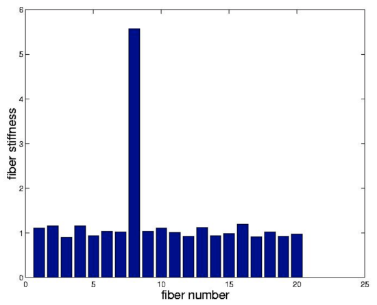
respectively. For the purpose of our example we suppose that each \(k_{j} = 1\) except \(k_{8} = 5\). We assemble \(A^{T}KA\) as in Chapter 2 and solve
\[A^{T}KAx^{j} = f^{j} \nonumber\]
with the help of the pseudoinverse. In order to impart some `reality' to this problem we taint each \(x^{j}\) with 10 percent noise prior to constructing \(B\)
\[B^{T}Bk = B^{T}f \nonumber\]
we note that Matlab solves this system when presented with k=B\f when BB is rectangular. We have plotted the results of this procedure in the link. The stiff fiber is readily identified.
Projections
From an algebraic point of view Equation is an elegant reformulation of the least squares problem. Though easy to remember it unfortunately obscures the geometric content, suggested by the word 'projection,' of Equation. As projections arise frequently in many applications we pause here to develop them more carefully. With respect to the normal equations we note that if \(\mathbb{N}(A) = \{0\}\) then
\[x = (A^{T}A)^{-1} A^{T} b \nonumber\]
and so the orthogonal projection of bb onto \(\mathbb{R}(A)\) is:
\[b_{R}= Ax \nonumber\]
\[= A (A^{T}A)^{-1} A^T b \nonumber\]
Defining
\[P = A (A^{T}A)^{-1} A^T \nonumber\]
takes the form \(b_{R} = Pb\). Commensurate with our notion of what a 'projection' should be we expect that \(P\) map vectors not in \(\mathbb{R}(A)\) onto \(\mathbb{R}(A)\) while leaving vectors already in \(\mathbb{R}(A)\) unscathed. More succinctly, we expect that \(Pb_{R} = b_{R}\) i.e., \(Pb_{R} = Pb_{R}\). As the latter should hold for all \(b \in R^{m}\) we expect that
\[P^2 = P \nonumber\]
We find that indeed
\[P^2 = A (A^{T}A)^{-1} A^T A (A^{T}A)^{-1} A^T \nonumber\]
\[= A (A^{T}A)^{-1} A^T \nonumber\]
\[= P \nonumber\]
We also note that the \(P\) is symmetric. We dignify these properties through
A matrix \(P\) that satisfies \(P^2 = P\) is called a projection. A symmetric projection is called an orthogonal projection.
We have taken some pains to motivate the use of the word 'projection.' You may be wondering however what symmetry has to do with orthogonality. We explain this in terms of the tautology
\[b = Pb−Ib \nonumber\]
Now, if \(P\) is a projection then so too is \(I-P\). Moreover, if \(P\) is symmetric then the dot product of \(b\).
\[\begin{align*} (Pb)^T(I-P)b &= b^{T}P^{T}(I-P)b \\[4pt] &= b^{T}(P-P^{2})b \\[4pt] &= b^{T} 0 b \\[4pt] &= 0 \end{align*}
i.e., \(Pb\) is orthogonal to \((I-P)b\). As examples of a nonorthogonal projections we offer
\[P = \begin{pmatrix} {1}&{0}&{0}\\ {\frac{-1}{2}}&{0}&{0}\\ {\frac{-1}{4}}&{\frac{-1}{2}}&{1} \end{pmatrix}\]
and \(I-P\). Finally, let us note that the central formula \(P = A (A^{T}A)^{-1} A^T\), is even a bit more general than advertised. It has been billed as the orthogonal projection onto the column space of \(A\). The need often arises however for the orthogonal projection onto some arbitrary subspace M. The key to using the old PP is simply to realize that every subspace is the column space of some matrix. More precisely, if
\[\{x_{1}, \cdots, x_{m}\} \nonumber\]
is a basis for MM then clearly if these \(x_{j}\) are placed into the columns of a matrix called \(A\) then \(\mathbb{R}(A) = M\). For example, if \(M\) is the line through \(\begin{pmatrix} {1}&{1} \end{pmatrix}^{T}\) then
\[P = \begin{pmatrix} {1}\\ {1} \end{pmatrix} \frac{1}{2} \begin{pmatrix} {1}&{1} \end{pmatrix} \nonumber\]
\[P = \frac{1}{2} \begin{pmatrix} {1}&{1}\\ {1}&{1} \end{pmatrix} \nonumber\]
is orthogonal projection onto \(M\).
Exercises
Gilbert Strang was stretched on a rack to lengths \(l = 6, 7, 8\) feet under applied forces of \(f = 1, 2, 4\) tons. Assuming Hooke's law \(l−L = cf\), find his compliance, \(c\), and original height, \(L\), by least squares.
With regard to the example of § 3 note that, due to the the random generation of the noise that taints the displacements, one gets a different 'answer' every time the code is invoked.
- Write a loop that invokes the code a statistically significant number of times and submit bar plots of the average fiber stiffness and its standard deviation for each fiber, along with the associated M--file.
- Experiment with various noise levels with the goal of determining the level above which it becomes difficult to discern the stiff fiber. Carefully explain your findings.
Find the matrix that projects \(\mathbb{R}^3\) onto the line spanned by \(\begin{pmatrix} {1}&{0}&{1} \end{pmatrix}^{T}\).
Find the matrix that projects \(\mathbb{R}^3\) onto the line spanned by \(\begin{pmatrix} {1}&{0}&{1} \end{pmatrix}^{T}\) and \(\begin{pmatrix} {1}&{1}&{-1} \end{pmatrix}^{T}\).
If \(P\) is the projection of \(\mathbb{R}^m\) onto a k--dimensional subspace \(M\), what is the rank of \(P\) and what is \(\mathbb{R}(P)\)?