2.7: The Exponential and Logarithm Functions

There are many applications in which it is necessary to find a function \(y\) of a variable \(t\) which has the property that

\[\frac{d y}{d t}=k y\]

for some constant real number \(k .\) Examples include modeling the growth of certain animal populations, where \(y\) is the size of the population at time \(t\) and \(k>0\) depends on the rate at which the population is growing, and describing the decay of a radioactive substance, where \(y\) is the amount of a radioactive material present at time \(t\) and \(k<0\) depends on the rate at which the element decays. We will first consider that case \(k=1 ;\) that is, we will look for a function \(y=f(t)\) with the property that \(f^{\prime}(t)=f(t)\).

2.7.1 The Exponential Function

Suppose \(f\) is a differential function on \((-\infty, \infty)\) with the property that \(f^{\prime}(t)=f(t)\) for all \(t\) (one may show that such a function does indeed exist, although we will not go into the details here). Now \(f^{\prime}(t)=f(t)\) implies, by the fundamental theorem of calculus, that

\[\int_{0}^{t} f(x) d x=\int_{0}^{t} f^{\prime}(x) d x=f(t)-f(0)\]

for all \(t .\) The value of \(f(0 \text { is arbitrary; we will find it convenient to take } f(0)=1\). That is, we are now looking for a function \(f\) which satisfies

\[f(t)=1+\int_{0}^{t} f(x) d x .\]

Suppose we divide \([0, t]\) into \(N\) subintervals of equal length \(\Delta x=\frac{t}{N},\) where \(N\) is a positive integer, and let \(x_{0}, x_{1}, x_{2}, \ldots, x_{N}\) be the endpoints of these intervals. Now for any \(i=1,2, \ldots, N,\) using \((2.7 .3),\)

\[\begin{aligned} f\left(x_{i}\right) &=1+\int_{0}^{x_{i}} f(x) d x \\ &=1+\int_{0}^{x_{i-1}} f(x) d x+\int_{x_{1-1}}^{x_{i}} f(x) d x \\ &=f\left(x_{i-1}\right)+\int_{x_{1-1}}^{x_{i}} f(x) d x .\end{aligned}\]

Moreover, for small \(\Delta x\),

\[\int_{x_{1-1}}^{x_{i}} f(x) d x \approx f\left(x_{i-1}\right) \Delta x,\]

and so we have

\[f\left(x_{i}\right) \approx f\left(x_{i-1}\right)+f\left(x_{i-1}\right) \Delta x=f\left(x_{i-1}\right)(1+\Delta x).\]

Hence we have

\[\begin{aligned} f\left(x_{0}\right) &=f(0)=1 \\ f\left(x_{1}\right) & \approx f\left(x_{0}\right)(1+\Delta x)=1+\Delta x \\ f\left(x_{2}\right) & \approx f\left(x_{1}\right)(1+\Delta x) \approx(1+\Delta x)^{2} \\ f\left(x_{3}\right) & \approx f\left(x_{2}\right)(1+\Delta x) \approx(1+\Delta x)^{3} \\ f\left(x_{4}\right) & \approx f\left(x_{3}\right)(1+\Delta x) \approx(1+\Delta x)^{4} \\ \vdots & \vdots \\ f\left(x_{N}\right) & \approx f\left(x_{N-1}\right)(1+\Delta x) \approx(1+\Delta x)^{N} \end{aligned}\]

Now \(x_{N}=t\) and \(\Delta x=\frac{t}{N},\) so we have

\[f(t) \approx\left(1+\frac{t}{N}\right)^{N}.\]

Moreover, if we followed the same procedure with \(N\) infinite and \(d x=\frac{t}{N},\) we should expect (although we have not proved)

\[f(t) \simeq\left(1+\frac{t}{N}\right)^{N}.\]

We will let \(e=f(1) .\) That is,

\[e=\operatorname{sh}\left(1+\frac{1}{N}\right)^{N},\]

where \(N\) is any positive infinite integer. We call \(e\) Euler's number. Now if \(t\) is any real number, then

\[f(t)=\left(1+\frac{t}{N}\right)^{N}=\left(\left(1+\frac{1}{\frac{N}{t}}\right)^{\frac{N}{t}}\right)^{t}=e^{t},\]

where we have used the fact that \(\frac{N}{t}\) is infinite since \(N\) is infinite and \(t\) is finite. (Note, however, that \(\frac{N}{t}\) is not an integer, as required in \((2.7 .16) .\) The statement is nevertheless true, but this is a detail which we will not pursue here.) Thus

the function

\[f(t)=e^{t}\]

has the property that \(f^{\prime}(t)=f(t),\) that is,

\[\frac{d}{d t} e^{t}=e^{t}.\]

In fact, one may show that \(f(t)=e^{t}\) is the only function for which \(f(0)=1\) and \(f^{\prime}(t)=f(t) .\) We call this function the exponential function, and sometimes write \(\exp (t)\) for \(e^{t} .\)

It has been shown that \(e\) is an irrational number. Although, like \(\pi,\) we may not express \(e\) exactly in decimal notation, we may use \((2.7 .16)\) to find approximations, replacing the infinite \(N\) with a large finite value for \(N .\) For example, with \(N=200,000,\) we find that

\[e \approx\left(1+\frac{1}{200000}\right)^{200000} \approx 2.71828,\]

which is correct to 5 decimal places.

Example \(\PageIndex{1}\)

If \(f(t)=e^{5 t},\) then \(f\) is the composition of \(h(t)=5 t\) and \(g(u)=e^{u} .\) Hence, using the chain rule,

\[f^{\prime}(t)=g^{\prime}(h(t)) h^{\prime}(t)=e^{5 t} \cdot 5=5 e^{5 t}.\] In general, if \(h(t)\) is differentiable, then, by the chain rule, \[\frac{d}{d t} e^{h(t)}=h^{\prime}(t) e^{h(t)}.\]

Example \(\PageIndex{2}\)

If \(f(x)=6 e^{-x^{2}},\) then

\[f^{\prime}(x)=-12 x e^{-x^{2}}.\]

Exercise \(\PageIndex{1}\)

Find the derivative of \(g(x)=12 e^{-7 x}\).

Answer

\(g^{\prime}(x)=-84 e^{-7 x}\)

Exercise \(\PageIndex{2}\)

Find the derivative of \(f(t)=3 t^{2} e^{-t}\).

Answer

\(f^{\prime}(t)=\left(6 t-3 t^{2}\right) e^{-t}\)

Example \(\PageIndex{3}\)

Let \(f(t)=e^{t}\) and \(g(t)=e^{-t} .\) since \(e^{t}>0\) for all \(t,\) we have \(f^{\prime}(t)=e^{t}>0\) and \(f^{\prime \prime}(t)=e^{t}>0\) for all \(t,\) and so \(f\) is increasing on \((-\infty, \infty)\) and the graph of \(f\) is concave upward on \((-\infty, \infty) .\) On the other hand, \(g^{\prime}(t)=-e^{-t}<0\) and \(g^{\prime \prime}(t)=e^{-t}>0\) for all \(t,\) so \(g\) is decreasing on \((-\infty, \infty)\) and the graph of \(g\) is concave upward on \((-\infty, \infty) .\) See Figure \(2.7 .1 .\)

Of course, it follows from \((2.7 .19)\) that \[\int e^{t} d t=e^{t}+c.\]

Example \(\PageIndex{4}\)

From what we have seen with the examples of derivatives above, we have

\[\int_{0}^{1} e^{-t} d t=-\left.e^{-t}\right|_{0} ^{1}=-e^{-1}+e^{0}=1-e^{-1} \approx 0.6321.\]

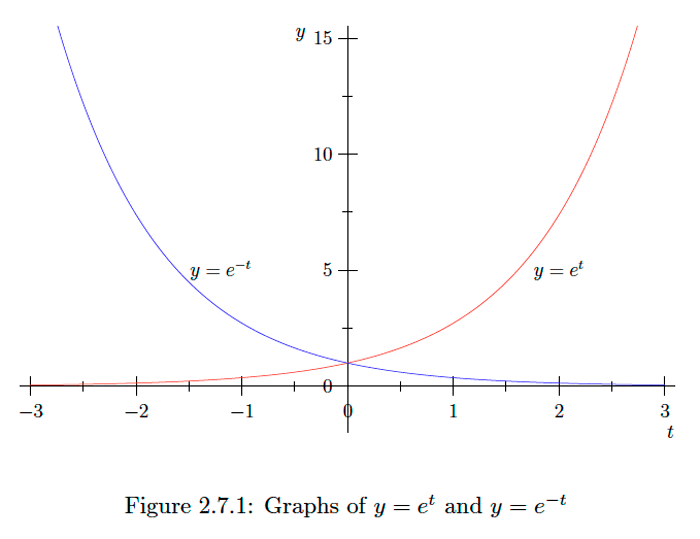
Example \(\PageIndex{5}\)

To evaluate

\[\int x e^{-x^{2}} d x,\] we will use the change of variable \[\begin{aligned} u &=-x^{2} \\ d u &=-2 x d x. \end{aligned}\] Then \[\int x e^{-^{2}} d x=-\frac{1}{2} \int e^{u} d u=-\frac{1}{2} e^{u}+c=-\frac{1}{2} e^{-x^{2}}+c.\]

Example \(\PageIndex{6}\)

To evaluate

\[\int x e^{-2 x} d x,\] we will use integration by parts: \[\begin{aligned} u &=x & & d v=e^{-2 x} d x \\ d u &=d x & & v=-\frac{1}{2} e^{-2 x} .\end{aligned}\] Then \[\int x e^{-2 x} d x=-\frac{1}{2} x e^{-2 x}+\frac{1}{2} \int e^{-2 x} d x=-\frac{1}{2} x e^{-2 x}-\frac{1}{4} e^{-2 x}+c.\]

Exercise \(\PageIndex{3}\)

Evaluate \(\int_{0}^{4} 5 e^{-2 x} d x\).

Answer

\(\int_{0}^{4} 5 e^{-2 x} d x=\frac{5}{2}-\frac{5}{2} e^{-8} \approx 2.4992\)

Exercise \(\PageIndex{4}\)

Evaluate \(\int_{0}^{1} x^{2} e^{-x^{3}} d x\).

Answer

\(\int_{0}^{1} x^{2} e^{-x^{3}} d x=\frac{1}{3}(1-e) \approx 0.2107\)

Exercise \(\PageIndex{5}\)

Evaluate \(\int x^{2} e^{-x} d x\).

Answer

\(\int x^{2} e^{-x} d x=-2 e^{-x}-2 x e^{-x}-x^{2} e^{-x}+c\)

Note that if \(y=a e^{k t},\) where \(a\) and \(k\) are any real constants, then

\[\frac{d y}{d t}=k a e^{k t}=k y.\]

That is, \(y\) satisfies the differential equation \((2.7 .1)\) with which we began this section. We will consider example applications of this equation after a discussion of the logarithm function, the inverse of the exponential function.

2.7.2 The Logarithm Function

The logarithm function is the inverse of the exponential function. That is, for a positive real number \(x, y=\log (x),\) read \(y\) is the logarithm of \(x,\) if and only if \(e^{y}=x .\) In particular, note that for any positive real number \(x,\)

\[e^{\log (x)}=x,\]

and for any real number \(x\),

\[\log \left(e^{x}\right)=x.\]

Also, since \(e^{0}=1,\) it follows that \(\log (1)=0\).

Since \(\log (x)\) is the power to which one must raise \(e\) in order to obtain \(x,\) logarithms inherit their basic properties from the properties of exponents. For example, for any positive real numbers \(x\) and \(y,\)

\[\log (x y)=\log (x)+\log (y)\]

since

\[e^{\log (x)+\log (y)}=e^{\log (x)} e^{\log (y)}=x y.\]

Similarly, for any positive real number \(x\) and any real number \(a\),

\[\log \left(x^{a}\right)=a \log (x)\]

since

\[e^{a \log (x)}=\left(e^{\log (x)}\right)^{a}=x^{a}.\]

Exercise \(\PageIndex{6}\)

Verify that for any positive real numbers \(x\) and \(y\),

\[\log \left(\frac{x}{y}\right)=\log (x)-\log (y).\] Note in particular that this implies that \[\log \left(\frac{1}{y}\right)=-\log (y).\] To find the derivative of the logarithm function, we first note that if \(y=\log (x),\) then \(e^{y}=x,\) and so \[\frac{d}{d x} e^{y}=\frac{d}{d x} x.\] Applying the chain rule, it follows that \[e^{y} \frac{d y}{d x}=1.\] Hence \[\frac{d y}{d x}=\frac{1}{e^{y}}=\frac{1}{x}.\]

Theorem \(\PageIndex{1}\)

For any real number \(x>0\),

\[\frac{d}{d x} \log (x)=\frac{1}{x}.\]

Example \(\PageIndex{7}\)

Since, for all \(x>0\)

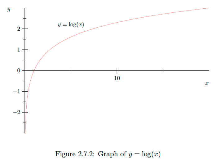
\[\frac{d}{d x} \log (x)=\frac{1}{x}>0\] and \[\frac{d^{2}}{d x^{2}} \log (x)=-\frac{1}{x^{2}}<0,\] the function \(y=\log (x)\) is increasing on \((0, \infty)\) and its graph is concave downward on \((0, \infty) .\) See Figure \(2.7 .2 .\)

Example \(\PageIndex{8}\)

If \(f(x)=\log \left(x^{2}+1\right),\) then, using the chain rule,

\[f^{\prime}(x)=\frac{1}{x^{2}+1} \frac{d}{d x}\left(x^{2}+1\right)=\frac{2 x}{x^{2}+1}.\]

Exercise \(\PageIndex{7}\)

Find the derivative of \(f(x)=\log (3 x+4)\).

Answer

\(f^{\prime}(x)=\frac{3}{3 x+4}\)

Exercise \(\PageIndex{8}\)

Find the derivative of \(y=(x+1) \log (x+1)\).

Answer

\(\frac{d y}{d x}=1+\log (x+1)\)

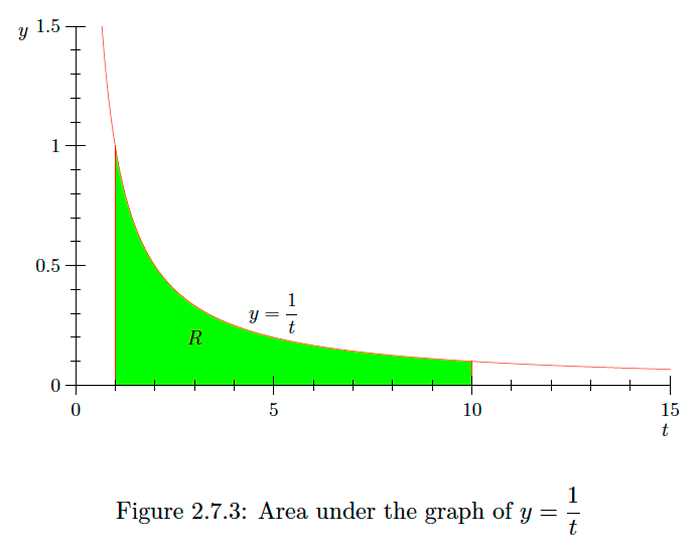
Using the fundamental theorem of calculus, it now follows that, for any \(x>0\),

\[\int_{1}^{x} \frac{1}{t} d t=\left.\log (t)\right|_{1} ^{x}=\log (x)-\log (1)=\log (x).\]

This provides a geometric interpretation of log(x) as the area under the graph of \(y=\frac{1}{t}\) from 1 to \(x\). For example, \(\log (10)\) is the area under the graph of \(y=\frac{1}{t}\) from \(1 \text { to } 10 \text { (see Figure } 2.7 .3) .\)

Example \(\PageIndex{9}\)

We may now complete the example, discussed in Example 2.5.8 and continued in Example 2.6 .19 , of finding the length \(L\) of the graph of \(y=x^{2}\) over the interval \([0,1] .\) In those examples we found that

\[L=\int_{0}^{1} \sqrt{1+4 x^{2}} d x=\frac{\sqrt{5}}{2}+\frac{1}{4} \int_{1}^{2+\sqrt{5}} \frac{1}{w} d w .\] Now we see that \[\int_{1}^{2+\sqrt{5}} \frac{1}{w} d w=\left.\log (w)\right|_{1} ^{2+\sqrt{5}}=\log (2+\sqrt{5}),\] and so \[L=\frac{\sqrt{5}}{2}+\frac{1}{4} \log (2+\sqrt{5}).\] Rounding to four decimal places, this gives us \(L \approx 1.4789,\) the same approximation we obtained in Example 2.5.8. Note, however, the advantage of having an exact impression for the answer: We may use the exact expression to easily approximate \(L\) to however many digits we desire, whereas we are unsure of the precision of our original approximate result, and would need to recalculate the approximating sum whenever we wanted to try to improve upon our accuracy. Moreover, our procedure for finding the expression for \(L\) may be extended easily to find an expression for the length of any segment of the parabola \(y=x^{2}\).

Example \(\PageIndex{10}\)

To evaluate

\[\int_{0}^{1} \frac{x}{1+x^{2}} d x,\] we first make the change of variable \[\begin{aligned} u &=1+x^{2} \\ d u &=2 x d x. \end{aligned}\] Then \[\int_{0}^{1} \frac{x}{1+x^{2}} d x=\frac{1}{2} \int_{1}^{2} \frac{1}{u} d u=\left.\frac{1}{2} \log (u)\right|_{1} ^{2}=\frac{\log (2)}{2}.\]

Example \(\PageIndex{11}\)

Evaluating

\[\int_{1}^{10} \log (x) d x\] provides an interesting application of integration by parts. If we let \[\begin{aligned} u &=\log (x) & & d v=d x \\ d u &=\frac{1}{x} d x & & v=x, \end{aligned}\] then \[\int_{1}^{10} \log (x) d x=\left.x \log (x)\right|_{1} ^{10}-\int_{1}^{10} d x=10 \log (10)-9.\]

Example \(\PageIndex{12}\)

We could use the change of variable \(u=3 x+2\) to evaluate

\[\int_{0}^{5} \frac{4}{3 x+2} d x,\] or just make the appropriate correction for the chain rule: \[\int_{0}^{5} \frac{4}{3 x+2} d x=\left.\frac{4}{3} \log (3 x+2)\right|_{0} ^{5}=\frac{4}{3}(\log (17)-\log (2))=\frac{4}{3} \log \left(\frac{17}{2}\right).\]

Exercise \(\PageIndex{9}\)

Evaluate \(\int_{0}^{2} \frac{1}{x+1} d x\).

Answer

\(\int_{0}^{2} \frac{1}{x+1} d x=\log (3)\)

Exercise \(\PageIndex{10}\)

Evaluate \(\int_{-1}^{2} \frac{x}{3 x^{2}+4} d x\).

Answer

\(\int_{-1}^{2} \frac{x}{3 x^{2}+4} d x=\frac{1}{6} \log \left(\frac{16}{7}\right)\)

Exercise \(\PageIndex{11}\)

Evaluate \(\int_{1}^{2} x \log (x) d x\).

Answer

\(\int_{1}^{2} x \log (x) d x=2 \log (2)-\frac{3}{4}\)

Exercise \(\PageIndex{12}\)

Evaluate \(\int_{-1}^{1} \sqrt{1+x^{2}} d x\).

Answer

\(\int_{-1}^{1} \sqrt{1+x^{2}} d x=\sqrt{2}+\log (1+\sqrt{2})\)

Exercise \(\PageIndex{13}\)

Evaluate \(\int_{-1}^{1} \frac{1}{\sqrt{1+x^{2}}} d x\).

Answer

\(\int_{-1}^{1} \frac{1}{\sqrt{1+x^{2}}} d x=2 \log (1+\sqrt{2})\)

It is now possible to extend the power rule for differentiating \(x^{n} .\) Suppose \(n \neq 0\) is a real number and note that, for \(x>0\),

\[x^{n}=e^{\log \left(x^{n}\right)}=e^{n \log (x)}.\]

Then

\[\begin{aligned} \frac{d}{d x} x^{n} &=\frac{d}{d x} e^{n \log (x)} \\ &=e^{n \log (x)} \frac{d}{d x} n \log (x) \\ &=\frac{n}{x} e^{n \log (x)} \\ &=\frac{n}{x} x^{n} \\ &=n x^{n-1} .\end{aligned}\]

Thus we have our final form of the power rule.

Theorem \(\PageIndex{1}\)

For any real number \(n \neq 0,\) if \(x>0\),

\[\frac{d}{d x} x^{n}=n x^{n-1}.\]

Example \(\PageIndex{13}\)

If \(f(x)=x^{\pi},\) then \(f^{\prime}(x)=\pi x^{\pi-1}\).

Exercise \(\PageIndex{14}\)

Find

\[\frac{d}{d x} \pi^{x}\] by first writing \(\pi^{x}=e^{x \log (\pi)} .\) How does this result compare with the result of the previous example?

Answer

\(\frac{d}{d x} \pi^{x}=(\log (\pi)) \pi^{x}\)

2.7.3 Some Applications

As mentioned at the beginning of this section, there are many applications in which one desires to find a function \(y\) which, for some constant \(k,\) satisfies the differential equation

\[\frac{d y}{d t}=k y .\]

Such an equation arises whenever the desired quantity grows, or decreases, at a rate which is proportional to its current value. As we saw above, a function of the form

\[y=\alpha e^{k t}\]

satisfies this equation for any real constant \(\alpha .\) Moreover, it may be shown that any solution must be of this form.

For example, \((2.7 .40)\) is used to model radioactive decay. That is, if one begins with \(y_{0}\) grams of a radioactive element and \(y\) is the amount of the element which remains after \(t\) years, then there is some constant \(k\) (which depends on the particular element being considered) for which

\[\frac{d y}{d t}=k y.\]

It follows that, for some real number \(\alpha\),

\[y=\alpha e^{k t}.\]

Since we are given that \(y=y_{0}\) when \(t=0,\) it follows that

\[y_{0}=y(0)=\alpha e^{0}=\alpha.\]

Hence

\[y=y_{0} e^{k t}.\]

Now suppose \(t_{1}<t_{2}\) are such that \(y\) at time \(t_{2}\) is one-half of \(y\) at time \(t_{1}\). Then

\[\frac{1}{2} y_{0} e^{k t_{1}}=y_{0} e^{k t_{2}}.\]

Thus

\[e^{k t_{1}}=2 e^{k t_{2}},\]

and so

\[2=\frac{e^{k t_{1}}}{e^{k t_{2}}}=e^{k\left(t_{1}-t_{2}\right)}.\]

Hence

\[\log (2)=\log \left(e^{k\left(t_{1}-t_{2}\right)}\right)=k\left(t_{1}-t_{2}\right),\]

from which it follows that

\[t_{2}-t_{1}=-\frac{\log (2)}{k}.\]

Note that the right-hand side of \((2.7 .50)\) does not depend on \(t_{1},\) and so the time required for one-half of a radioactive element to deeay does not depend on the initial amount of the element. We call this time the half-life of the element.

Typically the rate of decay of a radioactive element is expressed in terms of its half-life. From \((2.7 .50),\) we see that if the half-life of a particular element is \(T,\) then the decay rate of the element is

\[k=-\frac{\log 2}{T}.\]

Example \(\PageIndex{14}\)

Carbon-14 is a naturally occurring radioactive isotope of carbon with a half-life of 5730 years. A living organism will maintain constant level of carbon-\(14,\) which will begin to decay one the organism dies and is buried. Because of this, the amount of carbon-14 in the remains of an organism may be used to estimate its age. For example, suppose a piece of wood found buried at an archaeological site has \(14 \%\) of its original carbon-l4. If \(T\) is the number of years since the wood was buried and \(y_{0}\) is the original amount of carbon-14 in the wood, then

\[0.14 y_{0}=y_{0} e^{k T},\] where, from \((2.7 .51)\), \[k=-\frac{\log (2)}{5730}.\] It follows that \(0.14=e^{k T},\) and so \[k T=\log (0.14).\] Thus \[T=\frac{\log (0.14)}{k}=-\frac{5730 \log (0.14)}{\log (2)} \approx 16,253 \text { years. }\]

Exercise \(\PageIndex{15}\)

Suppose a piece of wood buried at an archaeological site has \(23 \%\) of its original carbon-\(14 .\) For how many years has the wood been buried?

Answer

\(12,149\) years

Exercise \(\PageIndex{16}\)

Suppose a radioactive element has a half-life of \(24,065\) years. How many years will it take for a given sample to decay to the point that only \(10 \%\) of the original amount remains?

Answer

\(79,942\) years

he differential equation \((2.7 .40)\) also serves in some situations as a simple model for population growth. Suppose, for example, that \(y\) is the size of a population of a certain species of animal over a specified habitat. In the absence of any extraneous limits on the size of the population (such as a limitation on the food supply, we would expect the rate of growth of the population to be proportional to the current population; that is, we would expect \(y\) to satisfy \((2.7 .40)\) for some constant \(k\). In particular, if \(y_{0}\), the size of the population at some initial time and \(y\) is the size of the population \(t\) year later, then

\[y=y_{0} e^{k t}.\]

Now suppose we know the population is \(y_{1}\) at some time \(t_{1}>0 .\) Then

\[y_{1}=y_{0} e^{k t_{1}},\]

and so, after dividing through by \(y_{0}\) and taking the logarithm of both sides,

\[k=\frac{1}{t_{1}} \log \left(\frac{y_{1}}{y_{0}}\right).\]

Example \(\PageIndex{15}\)

Suppose that a certain habitat initially holds a population of 1000 deer, and that five years later the population has grown to 1200 deer. If we let \(y\) be the size of the population after \(t\) years, and assuming no constraints on the growth of the population, we would have

\[y=1000 e^{k t},\] where \[k=\frac{1}{5} \log \left(\frac{1200}{1000}\right)=\frac{\log (1.2)}{5}.\] Then, for example, this model would predict a population of \[\begin{aligned} y(10) &=1000 e^{10 k} \\ &=1000 e^{2 \log (1.2)} \\ &=1000 e^{\log \left(1.2^{2}\right)} \\ &=(1000)(1.2)^{2} \\ &=1440 \text { deer } \end{aligned}\] after five more years.

If \(y\) is the size of a population of animals, we call the differential equation

\[\frac{d y}{d t}=k y,\]

and the resulting solution,

\[y=y_{0} e^{k t},\]

the natural growth model. Although often relatively accurate over small time intervals, this model is clearly unrealistic for any extended period of time as it predicts an unbounded growth. Even in the best of situations, other factors, such as availability of food and shelter, will eventually come into play.

The logistic model introduces a variation in the basic model \((2.7 .40)\) which factors in the limiting effect of space and food. In this case, we suppose that there is an upper bound, say \(M\), to the size of the population which the habitat can sustain and that the rate of growth of the population decreases as the size of the population approaches this limiting value. More precisely, let \(k\) be the natural rate of growth of the population, that is, the rate of growth if there are no constraining factors, or when the size of the population is small compared with \(M,\) and let \(y\) be the size of the population at time \(t .\) Then we suppose \(k\) is decreased by a factor of \(1-\frac{y}{M},\) that is, the proportion of room left for growth. The resulting differential equation for the logistic model is

\[\frac{d y}{d t}=k y\left(1-\frac{y}{M}\right)=\frac{k}{M} y(M-y)=\beta y(M-y),\]

where \(\beta=\frac{k}{M}\).

To solve \((2.7 .57),\) we first rewrite it using \(s\) for the independent variable, that is, as

\[\frac{d y}{d s}=\beta y(M-y),\]

and then divide through both sides by \(y(M-y)\) to obtain

\[\frac{1}{y(M-y)} \frac{d y}{d s}=\beta.\]

Next, we integrate both sides of this equation from 0 to some fixed time \(t:\)

\[\int_{0}^{t} \frac{1}{y(M-y)} \frac{d y}{d s} d s=\int_{0}^{t} \beta d s.\]

For the right hand side of \((2.7 .60),\) we have simply

\[\int_{0}^{t} \beta d s=\beta t.\]

For the left-hand side, we begin with the change of variable

\[\begin{aligned} u &=y \\ d u &=\frac{d y}{d s} d s, \end{aligned}\]

from which we obtain

\[\int_{0}^{t} \frac{1}{y(M-y)} \frac{d y}{d s} d s=\int_{y_{0}}^{y} \frac{1}{u(M-u)} d u,\]

where we have again used \(y_{0}\) to denote the size of the population at time \(s=0\) (and noting that \(y\) is the size of the population when \(s=t\) ). We assume that \(0<y_{0}<M\) and \(0<y<M ;\) that is, we assume that the populations involved are positive and do not exceed the maximum sustainable population.

To evaluate \((2.7 .63),\) we rely upon a result involving what are known as partial fraction decompositions: There exist real numbers \(A\) and \(B\) such that

\[\frac{1}{u(M-u)}=\frac{A}{u}+\frac{B}{M-u}.\]

To find \(A\) and \(B,\) we note that \((2.7 .64)\) implies that

\[\frac{1}{u(M-u)}=\frac{A(M-u)}{u(M-u)}+\frac{B u}{u(M-u)}=\frac{A(M-u)+B u}{u(M-u)}.\]

It follows that, for all values of \(u\),

\[1=A(M-u)+B u.\]

In particular, when \(u=0\) we have \(1=A M,\) and when \(u=M\) we have \(1=B M\).Hence

\[A=\frac{1}{M} \text { and } B=\frac{1}{M},\]

and so

\[\frac{1}{u(M-u)}=\frac{1}{M} \frac{1}{u}+\frac{1}{M} \frac{1}{M-u}.\]

Hence we now have

\[\begin{aligned} \int_{y_{0}}^{y} \frac{1}{u(M-u)} d u &=\frac{1}{M} \int_{y_{0}}^{y} \frac{1}{u} d u+\frac{1}{M} \int_{y_{0}}^{y} \frac{1}{M-u} d u \\ &=\left.\frac{1}{M} \log (u)\right|_{y_{0}} ^{y}-\left.\frac{1}{M} \log (M-u)\right|_{y_{0}} ^{y} \\ &=\frac{1}{M}\left(\log (y)-\log \left(y_{0}\right)-\log (M-y)\right.\\ &=\frac{1}{M} \log \left(\frac{y\left(M-y_{0}\right)}{y_{0}(M-y)}\right). \end{aligned}\]

Combining \((2.7 .60),(2.7 .61),\) and \((2.7 .69),\) we have

\[\beta M t=\log \left(\frac{y\left(M-y_{0}\right)}{y_{0}(M-y)}\right),\]

which now need to solve for \(y .\) To begin, exponentiate both sides to obtain

\[e^{\beta M t}=\frac{y\left(M-y_{0}\right)}{y_{0}(M-y)}.\]

It follows that

\[y\left(M-y_{0}\right)=e^{\beta M t} y_{0}(M-y)=y_{0} M e^{\beta M t}-y_{0} y e^{\beta M t},\]

and so

\[y_{0} M e^{\beta M t}=y\left(M-y_{0}\right)+y_{0} y e^{\beta M t}=\left(M+y_{0}\left(e^{\beta M t}-1\right)\right) y.\]

Thus

\[y=\frac{y_{0} M e^{\beta M t}}{\left(M+y_{0}\left(e^{\beta M t}-1\right)\right)}.\]

If we divide the numerator and denominator of the right-hand side by \(e^{\beta M t},\) we have

\[y=\frac{y_{0} M}{M e^{-\beta M t}+y_{0}-y_{0} e^{-\beta M t}},\]

from which we obtain our final form

\[y=\frac{y_{0} M}{y_{0}+\left(M-y_{0}\right) e^{-\beta M t}}.\]

Note that when \(t=0,(2.7 .76)\) reduces to \(y=y_{0},\) as it should given our initial condition, and when \(t\) is infinite, \(e^{-\beta M t} \simeq 0,\) and so \(y=M .\) Hence \(y_{0} \leq y<M\) for all \(t,\) with \(y\) approaching \(M\) as \(t\) grows.

Recalling that \(\beta=\frac{k}{M},\) where \(k\) is the natural rate of growth of the population, we may rewrite \((2.7 .76)\) as

\[y=\frac{y_{0} M}{y_{0}+\left(M-y_{0}\right) e^{-k t}}.\]

Example \(\PageIndex{16}\)

In our previous example, where \(y\) represented the number of deer in a certain habitat after \(t\) years, we found

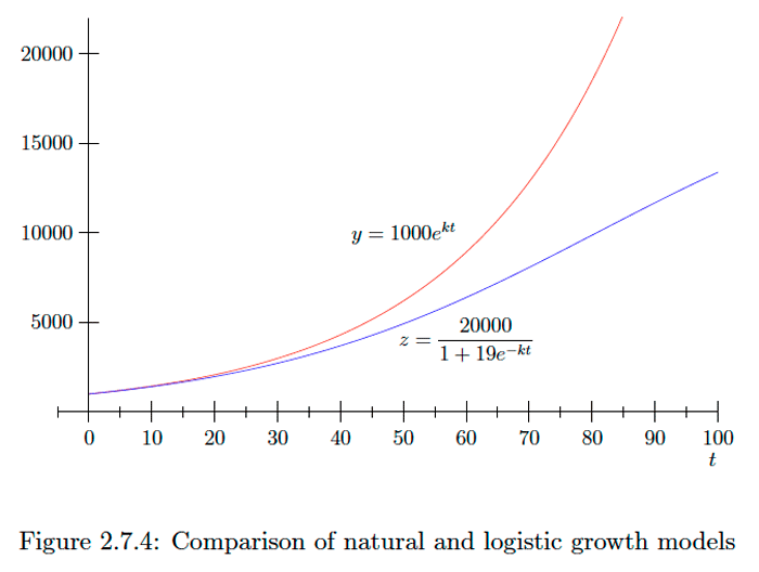
\[k=\frac{\log (1.2)}{5}.\] Now suppose the habitat ean support no more than \(20,000\) deer. Then the logistic model would give us \[z=\frac{(1000)(20000)}{1000+(20000-1000) e^{k t}}=\frac{20000}{1+19 e^{-k t}}\] for the number of deer after \(t\) years. After ten years, this model would predict a population of \[z(10)=\frac{20000}{1+19 e^{-10 k}} \approx 1409 \mathrm{deer},\] only slightly less than the 1440 predicted by the natural growth model. However, the differences between the two models become more pronounced with time. For example, after forty years, the natural growth model predicts \[y(40)=1000 e^{40 k} \approx 4300 \text { deer, }\]

while the logistic model predicts

\[z(40)=\frac{20000}{1+19 e^{-40 k}} \approx 3691 \mathrm{deer}\] and in 100 years, the natural growth model predicts \[y(100)=1000 e^{100 k} \approx 38338 \mathrm{ deer},\] while the logistic model predicts only \[z(100)=\frac{20000}{1+19 e^{-100 k}} \approx 13373 \text { deer. }\] Of course, over time the natural growth model predicts a population which grows without any bound, whereas the logistic model predicts that the population, while always increasing, will never surpass \(20,000 .\) See Figure \(2.7 .4 .\)

In evaluating \((2.7 .63)\) we made use of a partial fraction decomposition. More generally, suppose \(p\) and \(q\) are polynomials, the degree of \(p\) is less than the degree of \(q,\) and \(q\) factors completely into distinet linear factors, say,

\[q(x)=\left(a_{1} x+b_{1}\right)\left(a_{2} x+b_{2}\right) \cdots\left(a_{n} x+b_{n}\right).\]

Then it may be shown that there exist consants \(A_{1}, A_{2}, \ldots, A_{n}\) for which

\[\frac{p(x)}{q(x)}=\frac{A_{1}}{a_{1} x+b_{2}}+\frac{A_{2}}{a_{2} x+b_{2}}+\cdots+\frac{A_{n}}{a_{n} x+b_{n}}.\]

The evaluation of

\[\int_{a}^{b} \frac{p(x)}{q(x)} d x,\]

for any real numbers \(a\) and \(b\) for which \(q(x) \neq 0\) for all \(x\) in \([a, b],\) then follows easily.

Example \(\PageIndex{17}\)

To evaluate

\[\int_{0}^{1} \frac{x}{x^{2}-4} d x,\] we first note that, since \(x^{2}-4=(x-2)(x+2),\) there exist constants \(A\) and \(B\) for which \[\frac{x}{x^{2}-4}=\frac{A}{x-2}+\frac{B}{x+2}.\] It follows that \[\frac{x}{x^{2}-4}=\frac{A(x+2)+B(x-2)}{x^{2}-4},\] and so \[x=A(x+2)+B(x-2)\] for all values of \(x\). In particular, when \(x=2\) we have \(2=4 A,\) and when \(x=-2\) we have \(-2=-4 B .\) Hence \(A=\frac{1}{2}\) and \(B=\frac{1}{2},\) and so \[\frac{x}{x^{2}-4}=\frac{1}{2} \frac{1}{x-2}+\frac{1}{2} \frac{1}{x+2}.\] And so we have \[\int_{0}^{1} \frac{x}{x^{2}-4} d x=\frac{1}{2} \int_{0}^{1} \frac{1}{x-2} d x+\frac{1}{2} \int_{0}^{1} \frac{1}{x+2} d x.\] Now \[\frac{1}{2} \int_{0}^{1} \frac{1}{x+2} d x=\left.\frac{1}{2} \log (x+2)\right|_{0} ^{1}=\frac{1}{2}(\log (3)-\log (2)),\] but the first integral requires a bit more care because \(x-2<0\) for \(0 \leq x \leq 1\).If we make the change of variables, \[\begin{aligned} u &=-(x-2) \\ d u &=-d x, \end{aligned}\] then, since \(x-2=-u\), \[\begin{aligned} \frac{1}{2} \int_{0}^{1} \frac{1}{x-2} d x &=\frac{1}{2} \int_{2}^{1} \frac{1}{u} d u \\ &=-\frac{1}{2} \int_{1}^{2} \frac{1}{u} d u \\ &=-\left.\frac{1}{2} \log (u)\right|_{1} ^{2} \\ &=-\frac{1}{2} \log (2). \end{aligned}\] Hence \[\int_{0}^{1} \frac{x}{x^{2}-1} d x=\frac{1}{2}(\log (3)-\log (2))-\frac{1}{2} \log (2)=\frac{1}{2} \log (3)-\log (2).\]

Exercise \(\PageIndex{19}\)

Evaluate \(\int_{-2}^{2} \frac{1}{9-x^{2}} d x\).

Answer

\(\int_{-2}^{2} \frac{1}{9-x^{2}} d x=\frac{1}{3} \log (5)\)

Exercise \(\PageIndex{20}\)

Evaluate \(\int_{0}^{1} \frac{x+4}{x^{2}+3 x+2} d x\).

Answer

\(\int_{0}^{1} \frac{x+14}{x^{2}+3 x+2} d x=5 \log (2)-2 \log (3)\)