5.5: Aphids and Ladybugs, revisited

Aphids and Ladybugs, revisited

In Example 1.3, we asked when predation (by a ladybug) and growth rate exactly match for an aphid population. We did so by solving an equation of the form \(P(x)=G(x)\) for \(x\) the aphid density and \(G(x)=r x\) the aphid growth rate \((r>0)\), and \(P(x)\) the rate of predation of aphids by a ladybug. Our solution relied on the quadratic formula. Now consider the case that the predation rate is

\[P(x)=K \frac{x^{3}}{a^{3}+x^{3}}, \quad \text { where } \quad K, a>0 . \nonumber \]

In this case, steps shown in Example 1.3 lead to a cubic equation for \(x\), which is not easy to solve by pen and paper. This is a classic situation where Newton’s method proves useful.

Example 5.12 (Using Newton’s Method to solve the aphid-ladybug problem)

Set up the problem for obtaining the number of aphids at which predation by a ladybug and population growth of aphids balance. Convert the equation to a form for which Newton’s method is suitable. Then use Newton’s method to solve your problem. Assume that \(K=30\) aphids eaten per hour, \(a=20\) aphids, and \(r=0.5\) per hour. To get a reasonable initial guess, plot \(P(x)\) and \(G(x)\) on the same graph and determine roughly where they intersect.

Solution

The problem to be solved (assuming \(x \neq 0\) is

\[P(x)=G(x) \Rightarrow K \frac{x^{3}}{a^{3}+x^{3}}=r x \quad \Rightarrow \quad K \frac{x^{2}}{a^{3}+x^{3}}=r \nonumber \]

simplifying algebraically leads to the equation

\[K x^{2}=r\left(a^{3}+x^{3}\right) \Rightarrow r x^{3}-K x^{2}+r a^{3} \equiv f(x)=0 \nonumber \]

Having converted the problem into the form \(f(x)=0\), we can apply Newton’s method. We need the function and its derivative for Newton’s method formula,

\[\begin{aligned} & f(x)=r x^{3}-K x^{2}+r a^{3} \\ & f^{\prime}(x)=3 r x^{2}-2 K x \end{aligned} \nonumber \]

Using the numerical values for the constants, and examining the graph of the two functions \(P(x)\) and \(G(x)\), we find intersections at \(x=0\) and \(x_{0} \approx 10\). There is another intersection at \(x_{0} \approx 60\). To implement the method, we apply Newton’s formula,

\[x_{1}=x_{0}-\frac{f\left(x_{0}\right)}{f^{\prime}\left(x_{0}\right)}=x_{0}-\frac{\left(r x_{0}^{3}-K x_{0}^{2}+r a^{3}\right)}{3 r x_{0}^{2}-2 K x_{0}} \nonumber \]

with \(x_{0}=10\). Table \(5.3\) summarizes the convergence to the root \(x=\) 13.05407289 after four rounds of improvement using Newton’s method.

Table 5.3: Newton’s method applied to Example 5.12. We start with \(x_{0}=10\) as the initial approximation. Since \(x\) measures a density of aphids (e.g. average number per \(\mathrm{cm}^{2}\) ), it is reasonable to find a real valued solution (rather than an integer "number of aphids").

\(\boldsymbol{k}\)	\(\boldsymbol{x}_{k}\)	\(\boldsymbol{f}\left(\boldsymbol{x}_{k}\right)\)	\(\boldsymbol{f}^{\prime}\left(\boldsymbol{x}_{k}\right)\)	\(\boldsymbol{x}_{k+1}\)
\(\hdashline 0\)	10	\(1500.00\)	\(-450.00\)	\(13.33333333\)
1	\(13.33333333\)	\(-148.15\)	\(-533.33\)	\(13.05555556\)
2	\(13.05555556\)	\(-0.78\)	\(-527.66\)	\(13.05407294\)
3	\(13.05407294\)	\(0.00\)	\(-527.63\)	\(13.05407294\)
4	\(13.05407289\)	\(0.00\)	\(-527.63\)	\(13.05407294\)

Figure 5.9: The function \(P(x)\) superimposed on a graph of data from [Hassell et al., 1977].

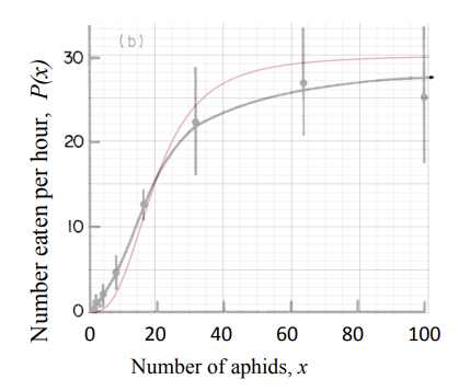
Examine this graph of the predation rate \(P(x)\) and the population growth rate \(G(x)\) to find reasonable initial guess(es) for points of intersection. (We look only for positive values, since \(x\) represents the number of aphids.) These will be used as value(s) for \(x_{0}\) in Newton’s method.

We conclude that at this aphid density, the aphid population would have a growth and a predation rate that exactly match. (Hence, we also expect that the aphid population would neither increase nor decrease.) What happens if growth and predation rates do not match? In such cases, we expect change to take place. How to analyze such situations will be the topic of a later chapter.

Why do we need to use Newton’s Method if we already solved the aphid -ladybug predation problem in Section 1.6.1?