1.3: The Cross Product
- Page ID
- 22920
As we noted in Section 1.1, there is no general way to define multiplication for vectors in \(\mathbb{R}^{n}\), with the product also being a vector of the same dimension, which is useful for our purposes in this book. However, in the special case of \(\mathbb{R}^{3}\) there is a product which we will find useful. One motivation for this product is to consider the following problem: Given two vectors \(\mathbf{x}=\left(x_{1}, x_{2}, x_{3}\right)\) and \(\mathbf{y}=\left(y_{1}, y_{2}, y_{3}\right)\) in \(\mathbb{R}^{3}\), not parallel to one another, find a third vector \(\mathbf{w}=\left(w_{1}, w_{2}, w_{3}\right)\) which is orthogonal to both \(\mathbf{x}\) and \(\mathbf{y}\). Thus we want \(\mathbf{w} \cdot \mathbf{x}=0\) and \(\mathbf{w} \cdot \mathbf{y}=0\), which means we need to solve the equations
\[x_1w_1 + x_2w_2+x_3w_3=0 \\ y_1w_1 + y_2w_2+y_3w_3=0 \label{1.3.1}\]
for \(w_1\), \(w_2\), and \(w_3\). Multiplying the first equation by \(y_3\) and the second by \(x_3\) gives us
\[x_1y_3w_1 + x_2y_3w_2 + x_3y_3w_3 = 0 \\ x_3y_1w_1 + x_3y_2w_2 + x_3y_3w_3 = 0 . \label{1.3.2} \]
Subtracting the second equation from the first, we have
\[ (x_1y_3-x_3y_1)w_1 + (x_2y_3-x_3y_2)w_2=0 . \label{1.3.3}\]
One solution of Equation \ref{1.3.3} is given by setting
\[w_1=x_2y_3-x_3y_2 \\ w_2=-(x_1y_3-x_3y_1) = x_3y_1-x_1y_3 . \label{1.3.4}\]
Finally, from the first equation in Equation \ref{1.3.1}, we now have
\[x_3w_3=-x_1(x_2y_3-x_3y_2)-x_2(x_3y_1-x_1y_3)=x_1x_3y_2-x_2x_3y_1 , \label{1.3.5}\]
from which we obtain the solution
\[w_3=x_1y_2-x_2y_1 . \label{1.3.6}\]
The choices made in arriving at Equation \ref{1.3.4} and \ref{1.3.6} are not unique, but they are the standard choices which define \(\mathbf{w}\) as the cross or vector product of \(\mathbf{x}\) and \(\mathbf{y}\).
Definition \(\PageIndex{1}\)
Given vectors \(\mathbf{x}=\left(x_{1}, x_{2}, x_{3}\right)\) and \(\mathbf{y}=\left(y_{1}, y_{2}, y_{3}\right)\) in \(\mathbb{R}^{3}\), the vector
\[ \mathbf{x}\times \mathbf{y}=(x_2y_3-x_3y_2,x_3y_1-x_1y_3,x_1y_2-x_2y_1)\]
is called the cross product, or vector product, of \(\mathbf{x}\) and \(\mathbf{y}\).
Example \(\PageIndex{1}\)
If \(\mathbf{x}=(1,2,3)\) and \(\mathbf{y}=(1,-1,1)\), then
\[\mathbf{x} \times \mathbf{y} = (2 + 3,3 − 1,−1 − 2) = (5,2,−3) . \nonumber \]
Note that
\[\mathbf{x} \cdot (\mathbf{x} \times \mathbf{y}) = 5+4-9=0 \nonumber\]
and
\[\mathbf{y} \cdot (\mathbf{x} \times \mathbf{y})=5-2-3=0 , \nonumber \]
showing that \(\mathbf{x} \perp (\mathbf{x} \times \mathbf{y})\) and \( \mathbf{y} \perp (\mathbf{x} \times \mathbf{y}) \) as claimed. It is also interesting to note that
\[\mathbf{y}\times \mathbf{x}=(-3-2,1-3,2+1)=(-5,-2,3)=-(\mathbf{x}\times \mathbf{y}) . \nonumber\]
This last calculation holds in general for all vectors \(\mathbf{x}\) and \(\mathbf{y}\) in \(\mathbb{R}^{3}\).
Proposition \(\PageIndex{1}\)
Suppose \(\mathbf{x}\), \(\mathbf{y}\), and \(\mathbf{z}\) are vectors in \(\mathbb{R}^3\) and \(\alpha\) is any real number. Then
\[\mathbf{x}\times \mathbf{y} = -(\mathbf{y} \times \mathbf{x}) , \]
\[\mathbf{x} \times (\mathbf{y}+\mathbf{z}) = (\mathbf{x} \times \mathbf{y}) + (\mathbf{x} \times \mathbf{z}) , \]
\[(\mathbf{x}+\mathbf{y}) \times \mathbf{z} = (\mathbf{x} \times \mathbf{z}) + (\mathbf{y} \times \mathbf{z}) , \]
\[ \alpha (\mathbf{x} \times \mathbf{y}) = (\alpha \mathbf{x}) \times \mathbf{y} = \mathbf{x} \times (\alpha \mathbf{y}) , \]
and
\[\mathbf{x} \times \mathbf{0} = \mathbf{0} . \]
Verification of these properties is straightforward and will be left to Exercise 10. Also, notice that
\[\mathbf{e}_1 \times \mathbf{e}_2 = \mathbf{e}_3 , \]
\[\mathbf{e}_2 \times \mathbf{e}_3 = \mathbf{e}_1 , \]
and
\[\mathbf{e}_3 \times \mathbf{e}_1 = \mathbf{e}_2 ; \]
that is, the cross product of two standard basis vectors is either the other standard basis vector or its negative. Moreover, note that in these cases the cross product points in the direction your thumb would point if you were to wrap the fingers of your right hand from the first vector to the second. This is in fact always true and results in what is known as the right-hand rule for the orientation of the cross product, as shown in Figure 1.3.1. Hence given two vectors \(\mathbf{x}\) and \(\mathbf{y}\), we can always determine the direction of \(\mathbf{x} \times \mathbf{y}\); to
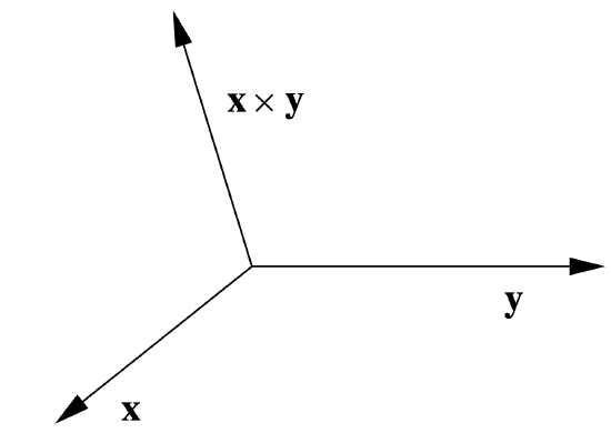
completely identify \(\mathbf{x} \times \mathbf{y}\) geometrically, we need only to know its length. Now if θ is the angle between \(\mathbf{x}\) and \(\mathbf{y}\), then
\begin{align}
\|\mathbf{x} \times \mathbf{y}\|^{2}=&\left(x_{2} y_{3}-x_{3} y_{2}\right)^{2}+\left(x_{3} y_{1}-x_{1} y_{3}\right)^{2}+\left(x_{1} y_{2}-x_{2} y_{1}\right)^{2} \nonumber \\
=& x_{2}^{2} y_{3}^{2}-2 x_{2} x_{3} y_{2} y_{3}+x_{3}^{2} y_{2}^{2}+x_{3}^{2} y_{1}^{2}-2 x_{1} x_{3} y_{1} y_{3}+x_{1}^{2} y_{3}^{2}+x_{1}^{2} y_{2}^{2} \nonumber \\
& \quad-2 x_{1} x_{2} y_{1} y_{2}+x_{2}^{2} y_{1}^{2} \nonumber \\
=&\left(x_{1}^{2}+x_{2}^{2}+x_{3}^{2}\right)\left(y_{1}^{2}+y_{2}^{2}+y_{3}^{2}\right)-\left(x_{1}^{2} y_{1}^{2}+x_{2}^{2} y_{2}^{2}+x_{3}^{2} y_{3}^{2}\right) \nonumber \\
& \quad-\left(2 x_{2} x_{3} y_{2} y_{3}+2 x_{1} x_{3} y_{1} y_{3}+2 x_{1} x_{2} y_{1} y_{2}\right) \nonumber \\
=&\left(x_{1}^{2}+x_{2}^{2}+x_{3}^{2}\right)\left(y_{1}^{2}+y_{2}^{2}+y_{3}^{2}\right)-\left(x_{1} y_{1}+x_{2} y_{2}+x_{3} y_{3}\right)^{2} \nonumber \\
=&\|\mathbf{x}\|^{2}\|\mathbf{y}\|^{2}-(\mathbf{x} \cdot \mathbf{y})^{2} \nonumber \\
=&\|\mathbf{x}\|^{2}\|\mathbf{y}\|^{2}-(\|\mathbf{x}\|\|\mathbf{y}\| \cos (\theta))^{2} \nonumber \\
=&\|\mathbf{x}\|^{2}\|\mathbf{y}\|^{2}\left(1-\cos ^{2}(\theta)\right) \nonumber \\
=&\|\mathbf{x}\|^{2}\|\mathbf{y}\|^{2} \sin ^{2}(\theta). \label{}
\end{align}
Taking square roots, and noting that \(\sin(\theta) \geq 0 \) since, by the definition of the angle between two vectors, \(0 \leq \theta \leq \pi \), we have the following result.
Proposition \(\PageIndex{2}\)
If θ is the angle between two vectors \(\mathbf{x}\) and \(\mathbf{y}\) in \(\mathbb{R}^{3}\), then
\[ \| \mathbf{x} \times \mathbf{y} \| = \| \mathbf{x} \| \| \mathbf{y} \| \sin (\theta) . \label{1.3.17} \]
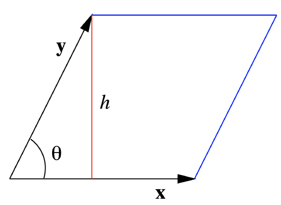
The last theorem has several interesting consequences. One of these comes from recognizing that if we draw a parallelogram with \(\mathbf{x}\) and \(\mathbf{y}\) as adjacent sides, as in Figure 1.3.2, then the height of the parallelogram is \(\| \mathbf{y} \| \sin(\theta)\), where θ is the angle between \(\mathbf{x}\) and \(\mathbf{y}\). Hence the area of the parallelogram is \(\| \mathbf{x} \| \| \mathbf{y} \| \sin(\theta)\), which by Equation \ref{1.3.17} is \(\| \mathbf{x} \times \mathbf{y} \|\).
Proposition \(\PageIndex{3}\)
Suppose \(\mathbf{x}\) and \(\mathbf{y}\) are two vectors in \(\mathbb{R}^{3}\). Then the area of the parallelogram which has \(\mathbf{x}\) and \(\mathbf{y}\) for adjacent sides is \(\| \mathbf{x} \times \mathbf{y} \| \).
Example \(\PageIndex{2}\)
Consider the parallelogram \(P\) with vertices at (0,0,0), (6,1,1), (8,5,2), and (2,4,1). Two adjacent sides are specified by the vectors \(\mathbf{x}=(6,1,1)\) and \(\mathbf{y}=(2,4,1)\) (see Figure 1.3.3), so the area of \(P\) is
\[\| \mathbf{x} \times \mathbf{y} \| = \|(1-4,2-6,24-2) \| = \| (-3,-4,22 \| = \sqrt{509} . \nonumber \]
See Figure 1.3.4 to see the relationship between \(\mathbf{x} \times \mathbf{y}\) and \(P\).
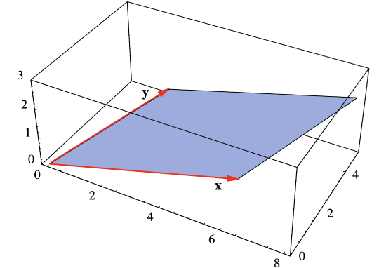
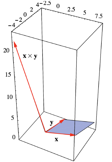
Figure 1.3.4 Parallelogram with adjacent sides \(\mathbf{x}=(6,1,1)\) and \(\mathbf{y}=(2,4,1)\)
Example \(\PageIndex{3}\)
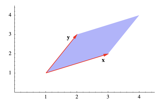
Consider the parallelogram \(P\) in the plane with vertices at (1,1,), (3,2), (4,4), and (2,3). Two adjacent sides are given by the vectors from (1,1) to (3,2), that is
\[\mathbf{x} = (3,2) - (1,1) = (2,1) , \nonumber \]
and from (1,1) to (2,3), that is,
\[\mathbf{y}=(2,3)-(1,1)=(1,2) . \nonumber\]
See Figure 1.3.5. However, since these vectors are in \(\mathbb{R}^2\), not in \(\mathbb{R}^3\), we cannot compute their cross product. To get around this, we consider the vectors \(\mathbf{w}=(2,1,0)\) and \(\mathbf{v}=(1,2,0)\) which are adjacent sides of the same parallelogram viewed as lying in \(\mathbb{R}^3\). Then the area of \(P\) is given by \[ \| \mathbf{w} × \mathbf{v} \| = \| (0,0,4 − 1) \| = \| (0,0,3)\| = 3 . \nonumber \]
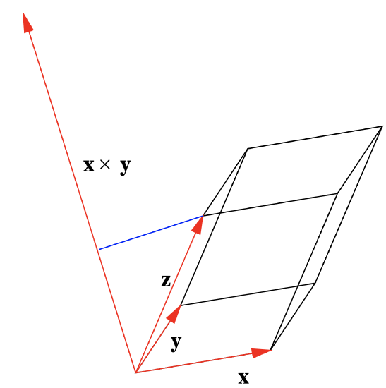
It is easy to extend the result of the previous theorem to computing the volume of a parallelepiped in \(\mathbb{R}^3\). Suppose \(\mathbf{x}\), \(\mathbf{y}\), and \(\mathbf{z}\) are adjacent edges of parallelepiped \(P\), as shown in Figure 1.3.6. Then the volume \(V\) of \(P\) is \(\| \mathbf{x} \times \mathbf{y} \| \), which is the area of the base, multiplied by the height of \(P\), which is the length of the projection of \(\mathbf{z}\) onto \(\mathbf{x} \times \mathbf{y}\). Since the latter is equal to
\[ \left| \mathbf{z} \cdot \frac{\mathbf{x} \times \mathbf{y}}{\| \mathbf{x} \times \mathbf{y} \|} \right| , \nonumber \]
we have
\[V = \| \mathbf{x} \times \mathbf{y} \| \left| z \cdot \frac{\mathbf{x} \times \mathbf{y}}{\| \mathbf{x} \times \mathbf{y} \|} \right| = \vert \mathbf{z} \cdot (\mathbf{x} \times \mathbf{y}) \vert . \]
Proposition \(\PageIndex{4}\)
The volume of a parallelepiped with adjacent edges \(\mathbf{x}\), \(\mathbf{y}\), and \(\mathbf{z}\) is \( \vert \mathbf{z} \cdot (\mathbf{x} \times \mathbf{y}) \vert \).
Definition \(\PageIndex{2}\)
Given three vectors \(\mathbf{x}\), \(\mathbf{y}\), and \(\mathbf{z}\) in \(\mathbb{R}^3\), the quantity \( \mathbf{z} \cdot (\mathbf{x} \times \mathbf{y}) \) is called the scalar triple product of \(\mathbf{x}\), \(\mathbf{y}\), and \(\mathbf{x}\).
Example \(\PageIndex{4}\)
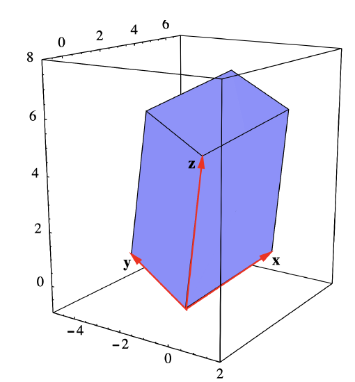
Let \(\mathbf{x}=(1,4,1)\), \(\mathbf{y}=(-3,1,1)\), and \(\mathbf{z}=(0,1,5)\) be adjacent edges of parallelepiped \(P\) (see Figure 1.3.7). Then \[\mathbf{x} \times \mathbf{y} = (4-1,-3-1,1+12) = (3,-4,13) , \nonumber \]
so
\[\mathbf{z} \cdot (\mathbf{x} \times \mathbf{y}) = 0-4+65 = 61. \nonumber \]
Hence the volume of \(P\) is 61.
The final result of this section follows from Equation \ref{1.3.17} and the fact that the angle between parallel vectors is either 0 or \(\pi\).
Proposition \(\PageIndex{5}\)
Vectors \(\mathbf{x}\) and \(\mathbf{y}\) in \(\mathbb{R}^3\) are parallel if and only if \(\mathbf{x} \times \mathbf{y}=\mathbf{0}\).
Note that, in particular, for any vector \(\mathbf{x}\) in \(\mathbb{R}^3\), \(\mathbf{x} \times \mathbf{x}=\mathbf{0}\).


